Let's first illustrate this with a relatively arbitrary example
by constructing a Bode plot of the transfer function
in equation 4.8 with
![]() given by
given by
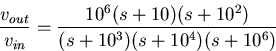 |
(73) |
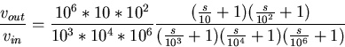 |
(74) |
![]() We now start plotting at frequency one decade less than the minimum pole
or zero, beginning by starting to draw a horizontal line at -80dB
from
We now start plotting at frequency one decade less than the minimum pole
or zero, beginning by starting to draw a horizontal line at -80dB
from ![]() to 10 rad/sec. At
to 10 rad/sec. At ![]() , we
encounter a zero, so we increase the slope to 20dB/dec. We continue
drawing a straight line with this slope until we reach
, we
encounter a zero, so we increase the slope to 20dB/dec. We continue
drawing a straight line with this slope until we reach ![]() ,where we encounter another zero, and thus increase the slope another 20dB/dec
to a total slope of 40dB/dec. We now continue along this slope until
we reach the first pole which is at
,where we encounter another zero, and thus increase the slope another 20dB/dec
to a total slope of 40dB/dec. We now continue along this slope until
we reach the first pole which is at ![]() where we decrease
the slope by 20dB/dec to 20dB/dec. We now continue at this slope
until we reach the second pole where decrease the slope another
20dB/dec to 0dB/dec. We then continue to draw this horizontal line
until we reach the final pole which will give a drop of 20dB/dec.
The resulting Bode plot, which is shown in Fig. 4.4.
where we decrease
the slope by 20dB/dec to 20dB/dec. We now continue at this slope
until we reach the second pole where decrease the slope another
20dB/dec to 0dB/dec. We then continue to draw this horizontal line
until we reach the final pole which will give a drop of 20dB/dec.
The resulting Bode plot, which is shown in Fig. 4.4.
It is important to notice that the largest value the Bode plot obtained was 0dB. This not an accident. It results because the original expression given by equation (4.8) was characteristic of passive circuits, which are circuits that do not have active gain elements such as transistors or op-amps.
Now, let's obtain a Bode plot for our original circuit of Fig. 4.2. The equation describing frequency-dependent gain of that circuit is given by equation 4.6. Let's factor out the poles to obtain a form similar to that of equation (4.9).
![\begin{displaymath}
\frac{v_{out}}{v_{in}}=
\left(\frac{-R_C\vert\vert R_L}{R_{E...
...2R_{in}C_1(R_L+R_C)C_2}{(sR_{in}C_1+1)(sC_2(R_L+R_C)+1)}\right]\end{displaymath}](img177.gif) |
(75) |
First let's plot the
frequency-dependent fractional part, and then add the constant coefficients.
Starting with the numerator, we have 2 zeros at ![]() , this gives
rise to a line with slope of 40dB/dec which is zero dB at
, this gives
rise to a line with slope of 40dB/dec which is zero dB at ![]() .
At
.
At ![]() the slope changes to 20dB/dec, and finally at
the slope changes to 20dB/dec, and finally at
![]() the slope decreases by another 20dB/dec to
become a horizontal line. Now we add 20log(RinC1)(C2(RL+Ro)).
to obtain the response of the passive part of the transfer function
only. Finally, we add the midband gain
the slope decreases by another 20dB/dec to
become a horizontal line. Now we add 20log(RinC1)(C2(RL+Ro)).
to obtain the response of the passive part of the transfer function
only. Finally, we add the midband gain ![]() to obtain a graph of the entire equation.
to obtain a graph of the entire equation.
We have just illustrated in detail the mechanics of drawing a Bode
plot. However, they can usually be drawn very quickly for the midband
to low frequency part of a response with the following approach.
Start by finding the highest frequency low-frequency pole, and
draw a horizontal line at that point for the midband gain.
Next, move to the left (direction of decreasing ![]() ,
and for each pole you encounter increase
your slope downward by 20dB/dec, and for each zero you encounter
decrease your downward slope by 20dB/dec. In a sense, it is
a very quick method of obtaining the same result
we described in detail above. The resulting Bode plot is sketched
in Fig. 4.5.
,
and for each pole you encounter increase
your slope downward by 20dB/dec, and for each zero you encounter
decrease your downward slope by 20dB/dec. In a sense, it is
a very quick method of obtaining the same result
we described in detail above. The resulting Bode plot is sketched
in Fig. 4.5.