Klauda Lab Simulation Wiki

Please Cite Source: Wildermuth, K.; Monje-Galvan, V.; Warburton, L. M.; Klauda, J. B., Effect of membrane lipid packing on stable binding of the ALPS peptide. Journal of Chemical Theory and Computation 2019, 15, 1418-1429. (https://pubs.acs.org/doi/10.1021/acs.jctc.8b00945)

This analysis focuses on the study of membrane lipid packing defects – areas of low density lipid packing on the surface of a membrane that expose the nonpolar core of the membrane. Packing defects arise from dispersion of membrane constituents due to external forces such as imposed surface tensions or chemical interactions with other molecules. The analysis of packing defects is useful when quantifying the membrane surface is of interest. For example, I used packing defect quantification to describe the dynamic binding event between the Osh4 ALPS-like peptide and a membrane surface, and to describe the effects of using the HMMM simulation technique.

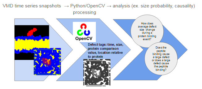
This process uses image processing techniques to identify packing defects in specially constructed images of the membrane surface.The process is broken into three steps illustrated in Figure 1: (1) constructing images in VMD, (2) identifying packing defects using Python and OpenCV, then (3) analyzing the results. Images produced in step 1 will look something like what is shown in Figure 1 where yellow “blobs” shown in the bottom image are the packing defects. In step 2, each packing defect on the membrane is identified as an individual object and tagged with descriptors such as time, size, and coordinates. The descriptors that are assigned to each defect can be expanded upon by future users. For step 3, I will present some analysis I have developed for my application, but the possibilities reach beyond what I describe here.

It is also worth noting that I developed this process to analyze the binding event of a peptide to a membrane, thus these scripts also incorporate identification and analysis of a protein in the simulation. The process can be simplified to study a membrane-only system (see notes in detailed instructions on where important changes should be made to study a membrane-only system).

Since this code has not been used by anyone but myself as of writing this, feel free to forward questions directly to me at kywildermuth@gmail.com.

Figure 1: Defect Analysis Workflow

Using the tachyon ray tracer in VMD, this script will produce a series of images that expose packing defects on the surface of a membrane from a MD trajectory. The images can be used for quantification and analysis of packing defects in a membrane and their relationship to a binding protein. This script produces a file architecture that is used in accompanied defect quantification and analysis scripts. Most of the user input changes will occur in this step.

The following files should be in the same directory (I will refer to the main directory as home)

1. DCD trajectory file: 1 DCD file containing the trajectory to be analyzed. It is recommended to use a DCD with a frame count corresponding to the number of images desired to be outputted (use merge DCD), although there are parameters available in this script for skipping frames in the DCD.
2. PSF file: associated PSF file for the trajectory.
3. defect_tachyon_scav.tcl: script called on by VMD
4. defect_tachyon.csh: c-shell script to submit job with SLURM and call VMD (default setup for DT1 operation)

1. Image files: Image files (default BMP) are saved within home using an automated directory architecture created by the script. Two image sets (protein and lipid) for each leaflet of the membrane are created, separated into two directories within home (top, bottom) for a total of four image sets. An optional side directory will be created if this image set is selected to be written.
2. Data files: text files are also created that include coordinate data to be used in associated analysis scripts.
   1. pbc_scale_dimnesions.dat: PBC coordinates of first frame of DCD
   2. PBC_coord.dat: contain PBC coordinates
   3. top_phos_Coord.dat, bot_phos_coord.dat: contain time series of average phosphate of each leaflet of the membrane
   4. prot_coord.dat, prot_minmax_coord.dat: contain time series associated with protein
   5. custom_coord.dat: time series for a defined custom selection (typically a protein residue of interest)
   6. VMD output file: will be written directly to home. Contains output lines from VMD operation. Useful for troubleshooting the script.

1. Many directions are contained in the script, defect_tachyon_scav.tcl.
2. Modify the CREATE REPRESENTATIONS section of the script to match the species in your system.
   1. The polar portion of some lipids have been predefined at the top of the script (ex. polar_PS, polar_PE). If a lipid in your system is not already listed, it must be defined. Default definition of polar is to include all atoms in the head group down to and including the second carbon in the lipid chain.
   2. If using an HMMM membrane, a selection exists to label all DCLE atoms nonpolar that are contained within the core of the membrane (default is -20Å<z<+20Å since some DCLE molecules escape the membrane)
   3. The default script draws the representations using the Quicksurf option. Quicksurf is relatively computationally expensive. For example, in my work I used quicksurf and image creation took a few days. I tried VDW spheres and it took less than an hour. I think using VDW representation will be OK (this needs to be confirmed) but make sure to use the same representation for all analysis to maintain consistency during analysis!
3. Modify the custom_sel variable if you want to track a specific selection during the trajectory. For example, if you wanted to track the TRP alpha carbon of a peptide, you could set custom_sel atom selection to resname TRP and name CA. The associated analysis scripts are constructed to read a custom_sel file, thus if you do not want to track a custom selection, just in the selection with something arbitrary and ignore its output.
4. set xsize, ysize: pixel dimensions of outputted images (default 600×600), recommended to keep 1:1 ratio.
5. set home: filepath to directory that contains input files
6. This script uses PBCTools to draw a box around the boundary of the system, centered on the protein.
   1. If no protein in system, can keep box centered on origin of system. The definition of the box needs to be edited if running the code on a system without a protein.
   2. Troubleshooting: f the protein wraps when viewed in VMD, uncomment the following line in the script to rewrap the membrane centered on the protein

    pbc wrap -centersel "protein" -center com -compound residue -all
 

1. Troubleshooting: if the box is hidden by the membrane when images are prepared, it might not be shifted in the direction of the camera enough. When the box is drawn, the option -shiftcenter moves the box. Increase the magnitude of the z coordinate in the appropriate direction if necessary.
2. Images are created using the tachyon ray tracer, which is a part of VMD but needs to be called separately. Default link to call tachyon is included in the file for DT1 but should be updated if not using DT1:

   render Tachyon $filename "/homes/jbklauda/vmd/vmd-1.9/lib/tachyon/tachyon_LINUXAMD64" $filename -lowshade -res 600 600 -format BMP -o $filename.bmp
 

1. the -lowshade option removes shade so that the image produced can be easily processed
2. the -res option can be changed if creating images larger than 600×600.

From command line in home, call defect_tachyon.csh. The cshell file calls VMD.

• The default file contains the filepath to the executable link for VMD on DT1, this should be changed if using a different system, or a newer version of VMD.
• The chsell script calls VMD without a display, so this process will run in the background
• The default file runs this process using the scavenger partition. You can change to another partition but this process runs fine on scavenger. I designed the code to pick up from where the process left off if it is cancelled in the middle of the run, so if you are knocked off, simply recall the cshell file and the job will continue from where it left off. Though I have never been knocked off scavenger.

Now we will run an image processing script on the prepared image sets. This step utilizes python and a computer vision library called OpenCV. Both softwares are available on DT1, and these directions will assume use of DT1 for operation of the analysis. Though in theory, this analysis can be run on any system with Python (and numpy) and OpenCV. Furthermore, I assume the use of OpenCV v.3.1.0 and Python v.2.7.8

A visual check of some of the images should be conducted before running the code to make sure things are in order. For example, make sure the green box is visible in the frame and, if there is a protein in the system, make sure the green box is centered on the protein. The protein should not wrap around the edge of the PBC. Protein images should contain only the protein, and lipid images should contain only the lipid.

1. blob_top.py, blob_bot.py: These are the python script files. Both files should be in home which contains the directories built by the previous VMD script. Note that the files are very similar, though blob_top.py runs analysis for the top leaflet of the membrane and blot_bot.py runs analysis for the bottom leaflet of the membrane
2. pbc_scale_dimensions.dat and image sets: these are built by the previous VMD script and are automatically structured appropriately.

1. local_defect_top.dat, local_defect_bot.dat: These files contain information about the packing defects closest to binding protein (if the file is edited to analyze membranes without proteins, this output file should be removed). The output files contain columns for frame number of the trajectory, area of defect below the protein (in Å^2), area of protein viewed from normal of z-plane (in Å^2), and a protein comparison value which is smaller when the local packing defect shape is similar to the protein shape (see openCV matchShapes function for more information
2. global_defect_top.dat, global_defect_bot.dat: These files contain information about the overall packing defect status of the entire system. The output files contain columns for frame number of the trajectory, area of the entire leaflet (in Å^2), and area of total defect on the leaflet (in Å^2).
3. defect_freq_area_top.dat, defect_freq_area_bot.dat: These files contain a list of all identified packing defects on their respective membrane leaflets. The columns from left to right are frame number that the defect appears in, the area of the defect (in Å^2), and the protein comparison value for that defect relative to the protein during the same frame.
   1. New defect properties can be defined in the script and added to this output file

1. All changes made in blob_top.py should be made in blob_bot.py and vice versa
2. Set variable parent_dir to the same as home used in the VMD script
3. Open pbc_scale_dimensions.dat and copy the values for the x and y coordinates of the box into the variables box_x and box_y into both blob_top.py and blob_bot.py. This is very important since this information is used to convert unit pixels to Å^2
4. Note: Packing defects with areas less than 1 Å^2 are ignored to clear up noise in the results. This threshold can be adjusted by changing the value in the definition of the is_contour_bad function

From the command line and while in home, load the two software modules and then simply call the python scripts:

module load python/2.7.8
module load opencv/3.1.0
python blob_top.py

• The code runs directly from the command line, and doesn't take more than a few minutes to complete. Updates of the code progress appear in the command line
• Both scripts can be run simultaneously to expedite the process (ex. from different PuTTy command lines)

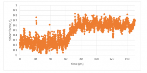
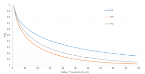
By completing steps 1 and 2, all packing defects have been identified. Now this information can be used to run analysis. Defect analysis will differ case-by-case. For example, if you are measuring defects to analyze a binding event of a protein, you might plot a time series of the local packing defect size relative to the protein area, which you would expect to increase when the peptide binds (Figure 2). If you want to determine how membrane properties differ between two simulations, you might run a statistical test on the set of identified packing defects of each simulation to see if there is a difference in a variable, such as the probability that a packing defect with an area larger than some threshold exists (Figure 3). These analysis can easily be conducted from the output files of the blob_top.py and blop_bot.py scripts. More complex analysis can also be created using the information provided from steps 1 and 2. Below is a process that outlines an example.

Figure 2: Local packing defect factor time series

Figure 3: Probability of a defect larger than a threshold existing for three different membrane types

Some proteins bind to membranes at large packing defects. One way to show that this is true is by comparing the probability of the peptide moving towards the membrane to the conditional probability of the peptide moving towards the membrane given that a large packing defect exists near the peptide (theoretical details are outlined in a paper published by our group). Using information from the packing defect analysis, we can run a script to compute the necessary probabilities to conduct this analysis.

The script truDiff.py can be run in the data_files directory created by the VMD script. This script will measure the minimum z-distance between the protein and the phosphate layer of a specified leaflet of the membrane. In the script, specify the final binding leaflet ('top' or 'bottom'), and the number of frames in the DCD (num_frame and prebind_limit). Execute the script from the command line by using the following code while in the data_files directory:

module load python/2.7.8
python truDiff.py

There will be a short prompt and the computation will complete quickly. An output file binding_distances.dat will be made which contains the necessary minimum binding distance time series, as well two other distance time series described in the script's header

Next, the script defect_peptide_frequency.py will count the number of times the peptide moves towards the membrane by a specified distance (m), how many instances a defect exists larger than a specified area (d), and how many times both of those instances occur simultaneously. These frequencies can be used to compute the probabilities and conditional probabilities described above. Options in the script allow the user to set the range of defect area and movement variable space, distance cutoffs (so you can analyze interactions only in a specific distance range between the membrane and the peptide), and trajectory cutoffs (so you can analyze interactions only in a specific time range, for example while the peptide is unbinded). Choose freq_path to be the local_defect data file for the leaflet of interest (typically the binding leaflet) and make sure the dist_path is set to the truDiff output file. Execute the script from the command line by using the following code while in the data_files directory:

 
module load python/2.7.8
python defect_peptide_frequency.py

• Note, the module load command does not have to be executed if the python module has already been loaded.
• The script will run in the command line, and takes a few minutes. The speed of the script is dependent primarily on the size of the movement variable sample space.
• The output file freq_stat_total.dat will contain counts of each event described above in a large table. Probabilities can be calculated from these tallies, and various results plotted (insert example excel sheet)