Part 5: Software Design Patterns
-
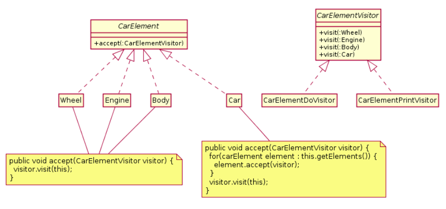
Working with the Visitor Design Pattern
-
Working with the Composite Hierarchy Design Pattern
-
Working with the Observer Design Pattern
Working with the Visitor Design Pattern
The visitor software design pattern provides a mechanism to
separate an algorithm (i.e. system functionality) from the object structure on which it operates.
The benefit of this separation is that new capabilities (or functions) can be added to
the class structure without changing its original structure.
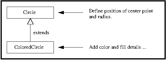
Example 18. In this example, print, price and draw visitors
visit a simple car model.
This example begins with a simple car data model containing
four wheels, a body, an engine, and the car component itself.
Access is provided for visitors.
Now let's see how this works for print, draw and price visitors.
/*
* ========================================================================
* input-sdp-visitor01.txt: Simulation of visitor design pattern ....
*
* Written By: Mark Austin January, 2017
* ========================================================================
*
import test.automobile.Car;
import test.automobile.CarDrawVisitor;
import test.automobile.CarPriceVisitor;
import test.automobile.CarPrintVisitor;
program ("Exercise Visitor Design Pattern") {
print "--- ========================================";
print "--- PART 01: Create car object ...";
print "--- ========================================";
car01 = Car();
print "--- ========================================";
print "--- PART 02: Visit car and draw elements ...";
print "--- ========================================";
cpv = CarPrintVisitor();
car01.accept( cpv );
print "--- ========================================";
print "--- PART 03: Visit car and draw elements ...";
print "--- ========================================";
cdv = CarDrawVisitor();
car01.accept( cdv );
print "--- ========================================";
print "--- PART 04: Visit car and compute cost ... ";
print "--- ========================================";
cpr = CarPriceVisitor();
car01.accept( cpr );
print "--- Total cost = ", cpr.getTotalPrice();
print "--- ========================================";
print "--- Finished !! ";
}
generates the textual output:
--- ========================================
--- PART 01: Create car object ...
--- ========================================
--- ========================================
--- PART 02: Visit car and draw elements ...
--- ========================================
Print: visiting front left wheel
Print: visiting front right wheel
Print: visiting rear left wheel
Print: visiting rear left wheel
Print: visiting body
Print: visiting engine
Print: visiting car
--- ========================================
--- PART 03: Visit car and draw elements ...
--- ========================================
Draw a wheel: front left ...
Draw a wheel: front right ...
Draw a wheel: rear left ...
Draw a wheel: rear left ...
Draw the body ...
Draw the engine ...
Draw my car ...
--- ========================================
--- PART 04: Visit car and compute cost ...
--- ========================================
Price: wheel = 1.00
Price: wheel = 1.00
Price: wheel = 1.50
Price: wheel = 1.50
Price: body = 5.00
Price: engine = 5.00
--- Total cost = [ 15.00, null]
--- =======================================================
--- Finished!
Points to note:
-
Each component of the car implements an CarElement interface, which in turn,
defines an accept method for entities that have implemented the CarElementVisitor interface.
-
The CarElementVisitor provides visit methods for each type of object found in
the car assembly, e.g., visit (Wheel item).
-
Thus, the details of print, draw and pricing are completely separated from the
Car Data Model by the common interfaces that they implement.
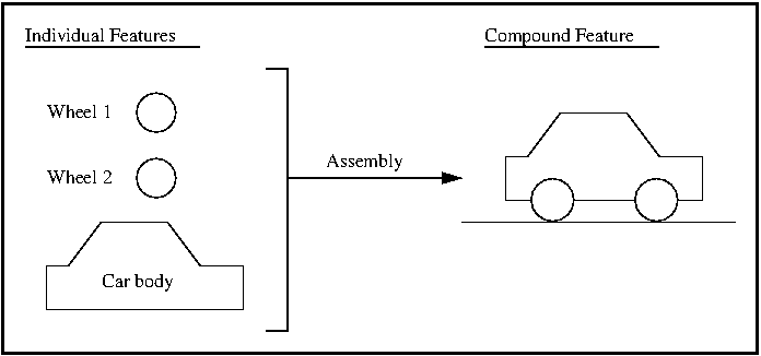
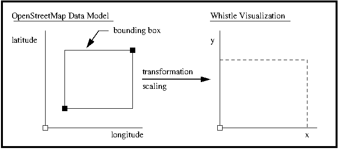
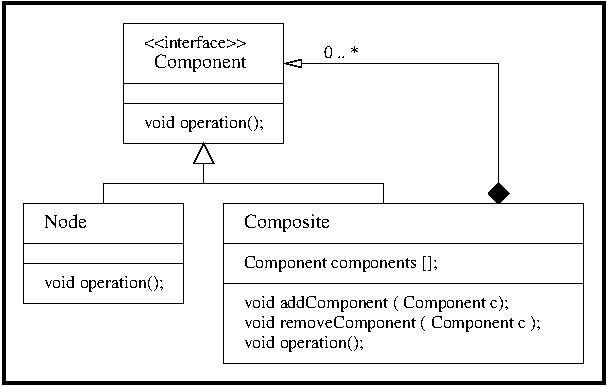
Working with the Composite Hierarchy Design Pattern
The composite hierarchy design pattern provides a flexible way to create
tree structures of arbitrary complexity,
while enabling every element in the structure to
operate with a uniform interface.
In a basic implementation of this pattern, the
arrangement of container and component classes is as follows:
Whistle extends this idea in the following ways:
The revised arrangement of Java classes is as follows:
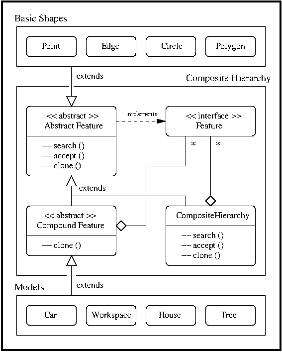
The centerpiece of this extension is the Feature interface:
public interface Feature extends Cloneable {
public BoundingEnvelope getBoundingEnvelope();
public void setName( String sName );
public String getName();
public void setX( Quantity dX );
public Quantity getX();
public void setY( Quantity dY );
public Quantity getY();
public void setPosition( Quantity dX, Quantity dY );
public void setHierarchyColor ( Color color );
public void setColor( Color c );
public void setColor( String c );
public Color getColor();
public void setFilledShape( Boolean b );
public boolean getFilledShape();
public void setSelection( Boolean b );
public boolean getSelection();
public void accept( FeatureElementVisitor visitor );
public void search( AffineTransform at, int dx, int dy );
}
Points to note:
-
The method getBoundingEnvelope() returns a rectangular box that bounds the feature,
a feature that is useful for quickly determing if two objects do not overlap.
-
The methods setX() and setY() position the feature in a coordinate system
local to its position in the composite hiearchy.
-
The methods getX() and getY() retrieve the coordinates ....
-
The method setPosition( dX, dY ) positions a feature at
coordinate (dX, dY).
-
Methods are provided for setting and getting color and
setting and getting selections.
-
The accept() method provides a way for visitors to traverse the composite hierarchy.
-
The search() method provides a way for things to be found.
-
The clone() method makes a copy of everything in the composite hierarchy.
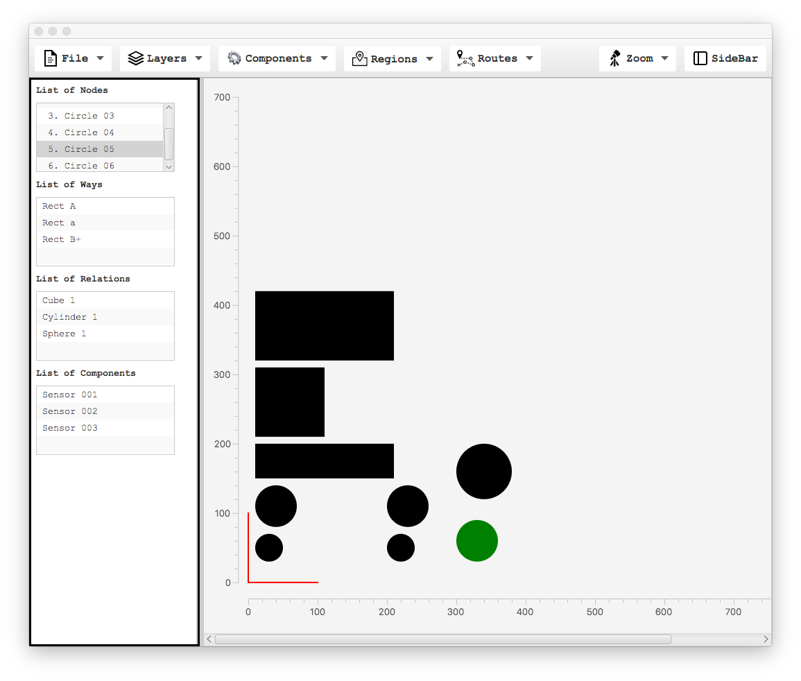
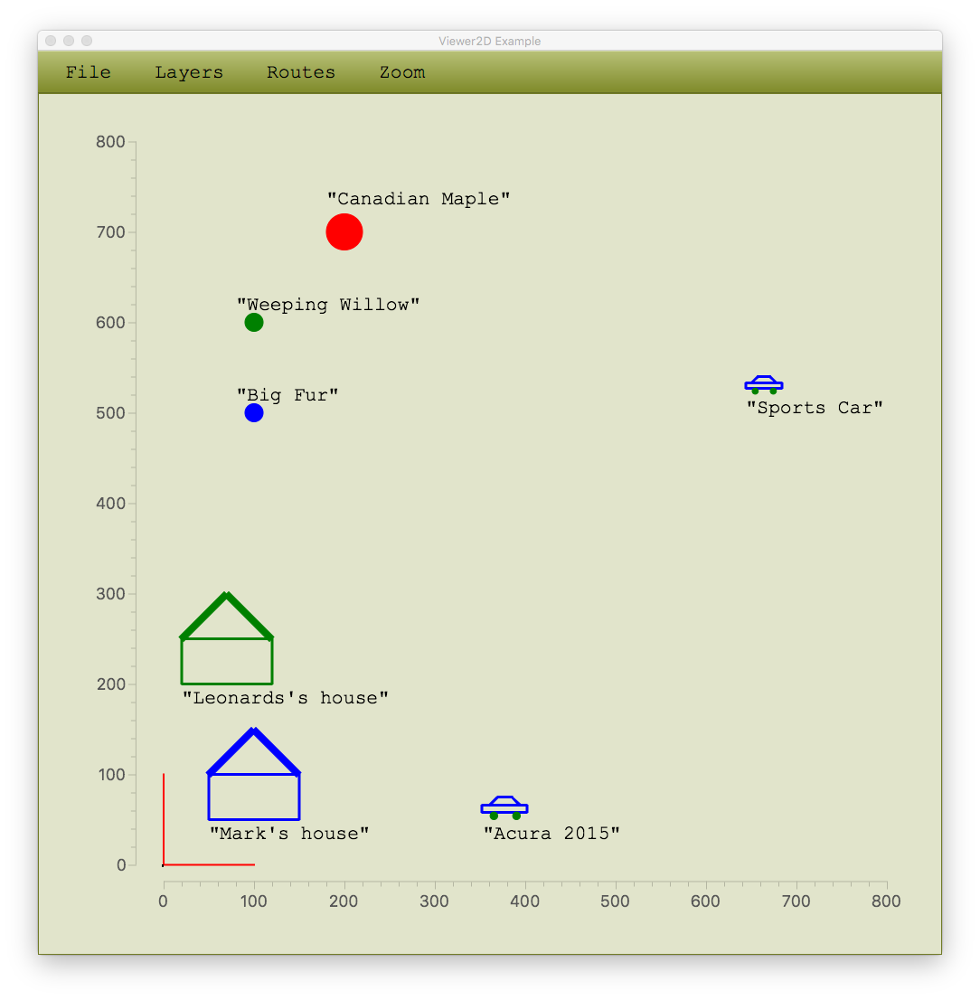
Example 19. Playing with compound models and workspaces of
manually assembled composite hierarchies.
// ========================================================================
// Experiment with models and composite hierarchies ....
//
// Written by: Mark Austin August 2014
// ========================================================================
import whistle.gui.Viewer2D;
import whistle.model.geometry.GridModel;
import whistle.model.WorkspaceModel;
import whistle.application.urban.TreeModel;
import whistle.application.urban.CarModel;
import whistle.application.urban.HouseModel;
program ("Composite Hierarchy Simulation") {
// Create and print model of an Acura 2015 and Sports Car ....
car01 = CarModel( 500 m, 50 m, 100 m );
car01.printMethods();
// Add data to car models, then print ...
car01.setName( "Acura 2015" );
car01.setColor("red");
car01.setDisplayName( true );
car02 = CarModel( 500 m, 350 m, 40 m );
car02.setName( "Sports Car" );
car02.setColor("red");
car02.setDisplayName( true );
print car01;
print car02;
// Create and print model of a house ....
house01 = HouseModel( 50 m, 50 m, 100 m );
house01.setName( "Mark's house" );
house01.setColor("blue");
house01.setDisplayName( true );
house02 = HouseModel( 20 m, 200 m, 200 m );
house02.setName( "Leonards's house" );
house02.setColor("green");
house02.setDisplayName( true );
print house01;
print house02;
// Create trees ....
tree01 = TreeModel( 100.0 m, 500 m, 10.0 m );
tree01.setName("Big Fur");
tree01.setColor("blue");
tree01.setFilledShape(true);
tree01.setDisplayName( true );
tree01.setTextOffSetX(-20.0);
tree01.setTextOffSetY( 25.0);
tree02 = TreeModel( 100.0 m, 600 m, 10.0 m );
tree02.setName("Weeping Willow");
tree02.setColor("green");
tree02.setFilledShape(true);
tree02.setDisplayName( true );
tree02.setTextOffSetX(-20.0);
tree02.setTextOffSetY( 25.0);
tree03 = TreeModel( 200.0 m, 700 m, 20.0 m );
tree03.setName("Canadian Maple");
tree03.setColor("red");
tree03.setFilledShape( true );
tree03.setDisplayName( true );
tree03.setTextOffSetX(-20.0);
tree03.setTextOffSetY( 42.0);
print tree01;
print tree02;
print tree03;
// Assemble composite hierarchy ....
ch = WorkspaceModel (0.0, 0.0, 0.0);
ch.setName ("Car and Trees");
ch.add ( car01 );
ch.add ( car02 );
ch.add ( house01 );
ch.add ( house02 );
ch.add ( tree01 );
ch.add ( tree02 );
ch.add ( tree03 );
ch.print();
// Workspace layer ....
workspacelayer = ch.getWorkspace();
// Create GridModel layer ....
grid = GridModel();
grid.setRange( 0 m, 0 m, 800 m, 800 m);
grid.setGridSize( 200 m );
grid.buildGrid();
gridlayer = grid.getWorkspace();
gridlayer.setColor("green");
// Build 2D viewer ...
jfx = Viewer2D();
jfx.addLayer( "Grid", gridlayer );
jfx.addLayer( "Stuff", workspacelayer );
// Setup and instantiate display ....
jfx.sleep( 1000 );
jfx.setSize( 1000, 1000 );
jfx.setXRange( 0, 800 );
jfx.setYRange( 0, 800 );
jfx.display();
jfx.sleep( 1000 );
print "--- ========================================== ";
print "--- Finished !!";
}
generates the graphic:
and the (slightly edited) textual output:
--- Begin Program: "Composite Hierarchy Simulation" ...
--- ==============================================================
--- Class diagnostics: whistle.model.urban.CarModel ...
--- ============================================================
// Methods declared in AbstractCompountFeature.java ....
Method name = setPerformance
Method return type = void
Parameters: double
Method name = setPrice
Method return type = void
Parameters: double
Method name = getPrice
Method return type = double
Parameters:
Method name = getPerformance
Method return type = double
Parameters:
// Methods declared in AbstractFeature.java ....
Method name = getName
Method return type = java.lang.String
Parameters:
Method name = setName
Method return type = void
Parameters: java.lang.String
Method name = getDisplayName
Method return type = boolean
Parameters:
Method name = setX
Method return type = void
Parameters: double
Method name = setX
Method return type = void
Parameters: whistle.Quantity
Method name = setY
Method return type = void
Parameters: whistle.Quantity
Method name = setY
Method return type = void
Parameters: double
Method name = setWidth
Method return type = void
Parameters: double
Method name = setWidth
Method return type = void
Parameters: whistle.Quantity
Method name = setHeight
Method return type = void
Parameters: whistle.Quantity
Method name = setHeight
Method return type = void
Parameters: double
Method name = getX
Method return type = whistle.Quantity
Parameters:
Method name = getY
Method return type = whistle.Quantity
Parameters:
Method name = getFilledShape
Method return type = boolean
Parameters:
Method name = getColor
Method return type = javafx.scene.paint.Color
Parameters:
Method name = setFilledShape
Method return type = void
Parameters: java.lang.Boolean
Method name = setDisplayName
Method return type = void
Parameters: java.lang.Boolean
Method name = getCoordinate
Method return type = whistle.model.Coordinate
Parameters:
Method name = getBoundingEnvelope
Method return type = whistle.model.BoundingEnvelope
Parameters:
Method name = setPosition
Method return type = void
Parameters: double, double
Method name = setPosition
Method return type = void
Parameters: whistle.Quantity, whistle.Quantity
Method name = setPosition
Method return type = void
Parameters: java.lang.Double, java.lang.Double
Method name = getHeight
Method return type = double
Parameters:
Method name = getWidth
Method return type = double
Parameters:
Method name = getArea
Method return type = double
Parameters:
Method name = setTextOffSetX
Method return type = void
Parameters: whistle.Quantity
Method name = setTextOffSetX
Method return type = void
Parameters: int
Method name = setTextOffSetY
Method return type = void
Parameters: whistle.Quantity
Method name = setTextOffSetY
Method return type = void
Parameters: int
Method name = getTextOffSetX
Method return type = double
Parameters:
Method name = getTextOffSetY
Method return type = double
Parameters:
Method name = setSelection
Method return type = void
Parameters: java.lang.Boolean
Method name = getSelection
Method return type = boolean
Parameters:
Method name = getShapeActive
Method return type = boolean
Parameters:
Method name = setHierarchyColor
Method return type = void
Parameters: javafx.scene.paint.Color
Method name = getPolygonString
Method return type = java.lang.String
Parameters:
Method name = setColor
Method return type = void
Parameters: javafx.scene.paint.Color
Method name = setColor
Method return type = void
Parameters: java.lang.String
// Methods declared above AbstractFeature.java ....
Method name = getClass
Method return type = java.lang.Class
Parameters:
--- ============================================================
---
--- Component: CarModel() ...
--- name = "Acura 2015"
--- (x,y) = (500.000000,50.000000)
--- height = 25.0
--- width = 50.0
--- Component: CarModel() ...
--- name = "Sports Car"
--- (x,y) = (500.000000,350.000000)
--- height = 20.0
--- width = 40.0
House Model: Name = "Mark's house"
Location (x,y) = ([ 50.00, null],[ 50.00, null])
House Model: Name = "Leonards's house"
Location (x,y) = ([ 20.00, null],[ 200.0, null])
Tree: Name = "Big Fur" ...
Coordinate(x,y) = (100.000000, 500.000000)
Tree shape filled --> true ...
Tree color --> [ #0000FF ] ...
Tree: Name = "Weeping Willow" ...
Coordinate(x,y) = (100.000000, 600.000000)
Tree shape filled --> true ...
Tree color --> [ #008000 ] ...
Tree: Name = "Canadian Maple" ...
Coordinate(x,y) = (200.000000, 700.000000)
Tree shape filled --> true ...
Tree color --> [ #FF0000 ] ...
// Print details of composite hierarchy ...
Start Composite Hierarchy: null
=================================================
Level = 1
-------------------------------------------------
Compound Feature: "Acura 2015"
----------------------------------
Local (x,y) = ( 500.0, 50.0 )
Global (x,y) = ( 500.0, 50.0 )
BoundingEnv[ x = (500.0-550.0) y = ( 50.0-75.0)]
----------------------------------
Point: (x,y) = (500.0, 58.3)
Point: (x,y) = (500.0, 66.7)
Point: (x,y) = (550.0, 66.7)
Point: (x,y) = (550.0, 58.3)
Edge: (x1,y1) = ( 500.00, 58.33)
: (x2,y2) = ( 500.00, 66.67)
: thickness = 2
Edge: (x1,y1) = ( 500.00, 66.67)
: (x2,y2) = ( 550.00, 66.67)
: thickness = 2
... details of car edges and points removed ...
Edge: (x1,y1) = ( 516.67, 75.00)
: (x2,y2) = ( 508.33, 66.67)
: thickness = 2
Circle( wheel01): (x,y) = ([ 512.5, null],[ 54.17, null]) radius = 4.16666667
Circle( wheel02): (x,y) = ([ 537.5, null],[ 54.17, null]) radius = 4.16666667
-------------------------------
Compound Feature: "Sports Car"
----------------------------------
Local (x,y) = ( 500.0, 350.0 )
Global (x,y) = ( 500.0, 350.0 )
BoundingEnv[ x = (500.0-540.0) y = ( 350.0-370.0)]
----------------------------------
Point: (x,y) = (500.0, 356.7)
... details of car edges and points removed ...
Circle( wheel01): (x,y) = ([ 510.0, null],[ 353.3, null]) radius = 3.333333335
Circle( wheel02): (x,y) = ([ 530.0, null],[ 353.3, null]) radius = 3.333333335
-------------------------------
Compound Feature: "Mark's house"
----------------------------------
Local (x,y) = ( 50.0, 50.0 )
Global (x,y) = ( 50.0, 50.0 )
BoundingEnv[ x = (50.0-150.0) y = ( 50.0-150.0)]
----------------------------------
Point: (x,y) = ( 50.0, 50.0)
Point: (x,y) = (150.0, 50.0)
Point: (x,y) = ( 50.0, 100.0)
Point: (x,y) = (150.0, 100.0)
Edge: (x1,y1) = ( 50.00, 50.00)
: (x2,y2) = ( 150.00, 50.00)
: thickness = 2
... details of house edges and points removed ...
Point: (x,y) = (100.0, 150.0)
-------------------------------
Compound Feature: "Leonards's house"
----------------------------------
... details of house edges and points removed ...
----------------------------------
Compound Feature: "Big Fur"
----------------------------------
Local (x,y) = ( 100.0, 500.0 )
Global (x,y) = ( 100.0, 500.0 )
BoundingEnv[ x = (90.0-110.0) y = ( 490.0-510.0)]
----------------------------------
Circle( base): (x,y) = ([ 100.0, null],[ 500.0, null]) radius = 10.0
----------------------------------
Compound Feature: "Weeping Willow"
----------------------------------
Local (x,y) = ( 100.0, 600.0 )
Global (x,y) = ( 100.0, 600.0 )
BoundingEnv[ x = (90.0-110.0) y = ( 590.0-610.0)]
----------------------------------
Circle( base): (x,y) = ([ 100.0, null],[ 600.0, null]) radius = 10.0
----------------------------------
Compound Feature: "Canadian Maple"
----------------------------------
Local (x,y) = ( 200.0, 700.0 )
Global (x,y) = ( 200.0, 700.0 )
BoundingEnv[ x = (180.0-220.0) y = ( 680.0-720.0)]
----------------------------------
Circle( base): (x,y) = ([ 200.0, null],[ 700.0, null]) radius = 20.0
-------------------------------
-------------------------------------------------
End level = 1
=================================================
Create Model of Workspace Grid
==============================
--- =======================================================
--- Finished!
Points to note:
Example 20. This example demonstrates systematic
assembly of a simple schematic for temperature control of two
rooms with HVAC equipment with a two-layer composite
hierarchy, i.e.,
The model employs and a variety of workspace transformations and
rotations to size and position the components in a desirable layout.
The workspace axes and orientations are illustrated with dark black arrows.
The abbreviated problem specification:
// ========================================================================
// Experiment with models and composite hierarchies ....
//
// Written by: Mark Austin June 2019
// ========================================================================
import whistle.gui.Viewer2D;
import whistle.model.WorkspaceModel;
import whistle.model.geometry.GridModel;
   import whistle.application.hvac.ChillerModel;
   import whistle.application.hvac.FanModel;
   import whistle.application.hvac.PipelineRegion;
   import whistle.application.hvac.PipelineModel;
   import whistle.application.hvac.SensorModel;
   import whistle.application.hvac.ControllerModel;
   import whistle.application.hvac.WallPlateModel;
program ("Demonstrate Composite Hierarchy Assembly") {
// ---------------------------------------------------------
// PART 1: HVAC Components ...
// =========================================================
// Controller model ...
controller01 = ControllerModel( 300.0, 660.0, 340.0, 140.0 );
controller01.setName( "HVAC Control" );
controller01.setColor( "greenyellow" );
controller01.setFilledShape(true);
controller01.setTextOffSetX(80);
controller01.setTextOffSetY(80);
// Chiller model ...
chiller01 = ChillerModel( 500, 480, 140);
chiller01.setName( "Chiller 01" );
chiller01.setFilledShape(true);
chiller01.setColor("greenyellow");
chiller01.setDisplayName( true );
chiller01.setTextOffSetX(0);
chiller01.setTextOffSetY(160);
// Fan model aligned with controller model ...
fan01 = FanModel( 760, 495, 80);
fan01.setName( "Fan 01" );
fan01.setColor("red");
fan01.setFilledShape(true);
fan01.setDisplayName(true);
fan01.setTextOffSetX( 0);
fan01.setTextOffSetY(-10);
fan02 = FanModel( 0, 0, 80);
fan02.setName( "Fan 02" );
fan02.setColor("red");
fan02.setFilledShape(true);
fan02.setDisplayName(true);
fan02.setTextOffSetX(0);
fan02.setTextOffSetY(100);
// Repositioned fan model rotated by PI/2 radians ...
ws01 = WorkspaceModel ( 840.0, 100.0, PI/2.0 );
ws01.add ( fan02 );
// Extract composite hierarchies from work spaces ...
chfan02 = ws01.getWorkspace();
// ----------------------------------------------------
// PART 2: Workspace model for Room 1 ...
// =========================================================
// Define geometry of centerlines for wall segments ...
wseg01 = PipelineRegion();
wseg01.add( 300.0, 285.0 );
wseg01.add( 15.0, 285.0 );
wseg01.add( 15.0, 15.0 );
wseg01.add( 300.0, 15.0 );
wseg02 = PipelineRegion();
wseg02.add( 330.0, 15.0 );
wseg02.add( 585.0, 15.0 );
wseg02.add( 585.0, 285.0 );
wseg02.add( 330.0, 285.0 );
// Transform wall centerlines into fill regions ...
width = 30;
room01pt1 = PipelineModel("Rm01, wall01");
room01pt1.setWidth( width );
room01pt1.build( wseg01 );
room01pt1.setDisplayName( false );
room01pt1.setColor( "blue" );
room01pt1.setFilledShape( true );
room01pt2 = PipelineModel("Rm01, wall02");
room01pt2.setWidth( width );
room01pt2.build( wseg02 );
room01pt2.setDisplayName( false );
room01pt2.setColor( "blue" );
room01pt2.setFilledShape( true );
// Wallplate models ...
wallplate01 = WallPlateModel( 300, 0, 30);
wallplate01.setName( "WP01" );
wallplate01.setFilledShape(true);
wallplate01.setColor("yellow");
wallplate01.setDisplayName( false );
wallplate02 = WallPlateModel( 300, 270, 30);
wallplate02.setName( "WP02" );
wallplate02.setFilledShape(true);
wallplate02.setColor("yellow");
wallplate02.setDisplayName( false );
// Sensor models ...
sensor01 = SensorModel( 150, 30, 10);
sensor01.setName( "S01" );
sensor01.setFilledShape(true);
sensor01.setColor("orange");
sensor01.setDisplayName( false );
... details of sensors removed ....
sensor02 = SensorModel( 150, 140, 10);
sensor03 = SensorModel( 150, 260, 10);
sensor04 = SensorModel( 450, 30, 10);
sensor05 = SensorModel( 450, 140, 10);
sensor06 = SensorModel( 450, 260, 10);
// --------------------------------------------------------
// Assemble components for Room 01 ...
// --------------------------------------------------------
wsroom01 = WorkspaceModel ( 100.0, 100.0, 0.0 );
wsroom01.add ( sensor01 );
wsroom01.add ( sensor02 );
wsroom01.add ( sensor03 );
wsroom01.add ( sensor04 );
wsroom01.add ( sensor05 );
wsroom01.add ( sensor06 );
wsroom01.add ( wallplate01 );
wsroom01.add ( wallplate02 );
wsroom01.add ( room01pt1 );
wsroom01.add ( room01pt2 );
// wsroom01.add ( room01pt1 );
chroom01 = wsroom01.getWorkspace();
// ----------------------------------------------------
// PART 3: Workspace model for Room 2 ...
// =========================================================
// Define geometry of centerlines for wall segments ...
wseg03 = PipelineRegion();
wseg03.add( 150.0, 285.0 );
wseg03.add( 15.0, 285.0 );
wseg03.add( 15.0, 15.0 );
wseg03.add( 585.0, 15.0 );
wseg03.add( 585.0, 285.0 );
wseg03.add( 450.0, 285.0 );
wseg04 = PipelineRegion();
wseg04.add( 180.0, 285.0 );
wseg04.add( 300.0, 285.0 );
wseg04.add( 420.0, 285.0 );
// Transform wall centerlines into fill regions ...
width = 30;
room02pt1 = PipelineModel("Rm01, wall01");
room02pt1.setWidth( width );
room02pt1.build( wseg03 );
room02pt1.setDisplayName( false );
room02pt1.setColor( "blue" );
room02pt1.setFilledShape( true );
room02pt2 = PipelineModel("Rm01, wall02");
room02pt2.setWidth( width );
room02pt2.build( wseg04 );
room02pt2.setDisplayName( false );
room02pt2.setColor( "blue" );
room02pt2.setFilledShape( true );
// Wallplate models ...
wallplate03 = WallPlateModel( 150, 270, 30);
wallplate03.setName( "WP01" );
wallplate03.setFilledShape(true);
wallplate03.setColor("yellow");
wallplate03.setDisplayName( false );
wallplate04 = WallPlateModel( 420, 270, 30);
wallplate04.setName( "WP02" );
wallplate04.setFilledShape(true);
wallplate04.setColor("yellow");
wallplate04.setDisplayName( false );
// Sensor models ...
sensor07 = SensorModel( 150, 140, 10);
sensor07.setName( "S07" );
sensor07.setFilledShape(true);
sensor07.setColor("orange");
sensor07.setDisplayName( false );
... details of sensors removed ...
sensor08 = SensorModel( 300, 140, 10);
sensor09 = SensorModel( 450, 140, 10);
// --------------------------------------------------------
// Assemble components for Room 02 ...
// --------------------------------------------------------
wsroom02 = WorkspaceModel ( 1200.0, 100.0, PI/2.0 );
wsroom02.add ( sensor07 );
wsroom02.add ( sensor08 );
wsroom02.add ( sensor09 );
wsroom02.add ( wallplate03 );
wsroom02.add ( wallplate04 );
wsroom02.add ( room02pt1 );
wsroom02.add ( room02pt2 );
chroom02 = wsroom02.getWorkspace();
// ====================================================================
// PART 4: Use pipes to connect chiller and fans to rooms ...
// ====================================================================
width = 2;
// Pipe 1: From Room 1 to Chiller ....
pipeline01 = PipelineRegion();
pipeline01.add( 400.0, 400.0 );
pipeline01.add( 400.0, 550.0 );
pipeline01.add( 500.0, 550.0 );
pipe01 = PipelineModel("pipe01");
pipe01.setWidth( width );
pipe01.build( pipeline01 );
pipe01.setDisplayName( false );
pipe01.setColor( "grey" );
pipe01.setFilledShape( true );
... details of pipe 02 through pipe 09 removed ...
pipe10 = PipelineModel("pipe08");
// ====================================================================
// PART 4: Use pipes to connect chiller and fans to rooms ...
// ====================================================================
width = 1;
// Wire 1: From HVAC Controller to Chiller ....
wireline01 = PipelineRegion();
wireline01.add( 640.0, 720.0 );
wireline01.add( 700.0, 720.0 );
wireline01.add( 700.0, 580.0 );
wireline01.add( 640.0, 580.0 );
wire01 = PipelineModel("wire01");
wire01.setWidth( width );
wire01.build( wireline01 );
wire01.setDisplayName( false );
wire01.setColor( "black" );
wire01.setFilledShape( true );
... details of wires 02 through wire05 removed ...
// ----------------------------------------------------
// PART 4: Assemble scene for HVAC workspace ...
// ----------------------------------------------------
hvac01 = WorkspaceModel ( 0.0, 0.0, 0.0 );
hvac01.add ( pipe01 ); hvac01.add ( pipe02 );
hvac01.add ( pipe03 ); hvac01.add ( pipe04 );
hvac01.add ( pipe05 ); hvac01.add ( pipe06 );
hvac01.add ( pipe07 ); hvac01.add ( pipe08 );
hvac01.add ( pipe09 ); hvac01.add ( pipe10 );
hvac01.add ( wire01 ); hvac01.add ( wire02 );
hvac01.add ( wire03 ); hvac01.add ( wire04 );
hvac01.add ( wire05 );
hvac01.add ( chroom01 );
hvac01.add ( chroom02 );
hvac01.add ( chiller01 );
hvac01.add ( chfan02 );
hvac01.add ( fan01 );
hvac01.add ( controller01 );
print "---";
print "--- ===============================================";
print "--- PRINT COMPOSITE HIERARCHY FOR HVAC WORKSPACE !!";
print "--- ===============================================";
print "---";
hvac01.print();
print "---";
print "--- ============================================ ";
print "--- BUILD 2D VIEWER AND INITIALIZE DISPLAY !! ...";
print "--- ============================================ ";
print "---";
// Extract composite hierarchy ...
hvaclayer01 = hvac01.getWorkspace();
// Build 2D viewer ...
jfx = Viewer2D();
jfx.addLayer( "HVAC Schematic", hvaclayer01 );
... details of viewer display removed ...
print "--- ================================================= ... ";
print "--- Finished !! ... ";
}
generates a two-layer composite hierarchy.
When a print visitor transitions through the composite
hierarchy the abbreviated output is as follows:
   --- ===============================================
   --- PRINT COMPOSITE HIERARCHY FOR HVAC WORKSPACE !!
   --- ===============================================

   Start Composite Hierarchy: null
   =================================================
   Level =  1
   -------------------------------------------------

   Compound Feature: pipe01 ...
   ------------------------------------------------
   Local  (x,y) = (   0.0,   0.0 )
   Global (x,y) = (   0.0,   0.0 )
   ------------------------------------------------
   Current Rotation (radians) = (   0.0000 )
                    (degrees) = (   0.0000 )
   ------------------------------------------------
   BoundingEnv[ x = (0.0--1.0) y = ( 0.0--1.0)]
   ------------------------------------------------
   SimplePolygon: name = P01 ...
   ================================================= ...
   --- width  =   101.00 ...
   --- height =   151.00 ...
   ================================================= ...
   --- Point  1: (x,y) = (  399.00,   400.00) ...
   --- Point  2: (x,y) = (  399.00,   551.00) ...
   --- Point  3: (x,y) = (  500.00,   551.00) ...
   --- Point  4: (x,y) = (  500.00,   549.00) ...
   --- Point  5: (x,y) = (  401.00,   549.00) ...
   --- Point  6: (x,y) = (  401.00,   400.00) ...
   ================================================= ...

   ... details of pipes removed ...

   Compound Feature: wire01 ...
   ------------------------------------------------
   Local  (x,y) = (   0.0,   0.0 )
   Global (x,y) = (   0.0,   0.0 )
   ------------------------------------------------
   Current Rotation (radians) = (   0.0000 )
                    (degrees) = (   0.0000 )
   ------------------------------------------------
   BoundingEnv[ x = (0.0--1.0) y = ( 0.0--1.0)]
   ------------------------------------------------
   SimplePolygon: name = P01 ...
   ================================================= ...
   --- width  =    60.50 ...
   --- height =   141.00 ...
   ================================================= ...
   --- Point  1: (x,y) = (  640.00,   720.50) ...
   --- Point  2: (x,y) = (  700.50,   720.50) ...
   --- Point  3: (x,y) = (  700.50,   579.50) ...
   --- Point  4: (x,y) = (  640.00,   579.50) ...
   --- Point  5: (x,y) = (  640.00,   580.50) ...
   --- Point  6: (x,y) = (  699.50,   580.50) ...
   --- Point  7: (x,y) = (  699.50,   719.50) ...
   --- Point  8: (x,y) = (  640.00,   719.50) ...
   ================================================= ...

   ... details of wires removed ...

   Start Composite Hierarchy: null
   =================================================
   Level =  2
   -------------------------------------------------

   Compound Feature: S01 ...
   ------------------------------------------------
   Local  (x,y) = ( 150.0,  30.0 )
   Global (x,y) = ( 250.0, 130.0 )
   ------------------------------------------------
   Current Rotation (radians) = (   0.0000 )
                    (degrees) = (   0.0000 )
   ------------------------------------------------
   BoundingEnv[ x = (150.0-160.0) y = ( 30.0-40.0)]
   ------------------------------------------------
   Edge: (x1,y1) = (    150.00,      30.00)
       : (x2,y2) = (    160.00,      30.00)
       : thickness =   2

   Edge: (x1,y1) = (    160.00,      30.00)
       : (x2,y2) = (    160.00,      40.00)
       : thickness =   2

   Edge: (x1,y1) = (    160.00,      40.00)
       : (x2,y2) = (    150.00,      40.00)
 ]     : thickness =   2

   Edge: (x1,y1) = (    150.00,      40.00)
       : (x2,y2) = (    150.00,      30.00)
       : thickness =   2

   Edge: (x1,y1) = (    150.00,      30.00)
       : (x2,y2) = (    160.00,      40.00)
       : thickness =   1

   Edge: (x1,y1) = (    160.00,      30.00)
       : (x2,y2) = (    150.00,      40.00)
       : thickness =   1

   Point: (x,y) = (150.0,  30.0)
   Point: (x,y) = (160.0,  30.0)
   Point: (x,y) = (160.0,  40.0)
   Point: (x,y) = (150.0,  40.0)
   ------------------------------------------------

   ... details of sensor output removed ...

   Compound Feature: WP01 ...
   ------------------------------------------------
   Local  (x,y) = ( 300.0,   0.0 )
   Global (x,y) = ( 400.0, 100.0 )
   ------------------------------------------------
   Current Rotation (radians) = (   0.0000 )
                    (degrees) = (   0.0000 )
   ------------------------------------------------
   BoundingEnv[ x = (300.0-330.0) y = ( 0.0-30.0)]
   ------------------------------------------------
   Edge: (x1,y1) = (    300.00,       0.00)
       : (x2,y2) = (    330.00,       0.00)
       : thickness =   4

   ... details of wall plate removed ...

   Edge: (x1,y1) = (    330.00,      22.50)
       : (x2,y2) = (    300.00,      22.50)
       : thickness =   2

   Point: (x,y) = (300.0,   0.0)
   Point: (x,y) = (330.0,   0.0)
   Point: (x,y) = (330.0,   7.5)
   Point: (x,y) = (330.0,  15.0)
   Point: (x,y) = (330.0,  22.5)
   Point: (x,y) = (330.0,  30.0)
   Point: (x,y) = (300.0,  30.0)
   Point: (x,y) = (300.0,  22.5)
   Point: (x,y) = (300.0,  15.0)
   Point: (x,y) = (300.0,   7.5)
   ------------------------------------------------

   ...  wall plates removed ...

   Compound Feature: Rm01, wall01 ...
   ------------------------------------------------
   Local  (x,y) = (   0.0,   0.0 )
   Global (x,y) = ( 100.0, 100.0 )
   ------------------------------------------------
   Current Rotation (radians) = (   0.0000 )
                    (degrees) = (   0.0000 )
   ------------------------------------------------
   BoundingEnv[ x = (0.0--1.0) y = ( 0.0--1.0)]
   ------------------------------------------------
   SimplePolygon: name = P01 ...
   ================================================= ...
   --- width  =   300.00 ...
   --- height =   300.00 ...
   ================================================= ...
   --- Point  1: (x,y) = (  300.00,   270.00) ...
   --- Point  2: (x,y) = (   30.00,   270.00) ...
   --- Point  3: (x,y) = (   30.00,    30.00) ...
   --- Point  4: (x,y) = (  300.00,    30.00) ...
   --- Point  5: (x,y) = (  300.00,     0.00) ...
   --- Point  6: (x,y) = (   -0.00,     0.00) ...
   --- Point  7: (x,y) = (    0.00,   300.00) ...
   --- Point  8: (x,y) = (  300.00,   300.00) ...
   ================================================= ...

   Compound Feature: Rm01, wall02 ...
   ------------------------------------------------
   Local  (x,y) = (   0.0,   0.0 )
   Global (x,y) = ( 100.0, 100.0 )
   ------------------------------------------------
   Current Rotation (radians) = (   0.0000 )
                    (degrees) = (   0.0000 )
   ------------------------------------------------
   BoundingEnv[ x = (0.0--1.0) y = ( 0.0--1.0)]
   ------------------------------------------------
   SimplePolygon: name = P01 ...
   ================================================= ...
   --- width  =   270.00 ...
   --- height =   300.00 ...
   ================================================= ...
   --- Point  1: (x,y) = (  330.00,    30.00) ...
   --- Point  2: (x,y) = (  570.00,    30.00) ...
   --- Point  3: (x,y) = (  570.00,   270.00) ...
   --- Point  4: (x,y) = (  330.00,   270.00) ...
   --- Point  5: (x,y) = (  330.00,   300.00) ...
   --- Point  6: (x,y) = (  600.00,   300.00) ...
   --- Point  7: (x,y) = (  600.00,     0.00) ...
   --- Point  8: (x,y) = (  330.00,     0.00) ...
   ================================================= ...

   -------------------------------------------------
   End level =  2
   =================================================

   Start Composite Hierarchy: null
   =================================================
   Level =  2
   -------------------------------------------------

   ... details of sensors S07 -- S09 removed ...

   ... details of wall plates WP01 and WP02 removed ...

   Compound Feature: Rm02, wall01 ...
   ------------------------------------------------
   Local  (x,y) = (   0.0,   0.0 )
   Global (x,y) = ( 1200.0, 100.0 )
   ------------------------------------------------
   Current Rotation (radians) = (   1.5708 )
                    (degrees) = (  90.0000 )
   ------------------------------------------------
   BoundingEnv[ x = (0.0--1.0) y = ( 0.0--1.0)]
   ------------------------------------------------
   SimplePolygon: name = P01 ...
   ================================================= ...
   --- width  =   600.00 ...
   --- height =   300.00 ...
   ================================================= ...
   --- Point  1: (x,y) = (  150.00,   270.00) ...
   --- Point  2: (x,y) = (   30.00,   270.00) ...
   --- Point  3: (x,y) = (   30.00,    30.00) ...
   --- Point  4: (x,y) = (  570.00,    30.00) ...
   --- Point  5: (x,y) = (  570.00,   270.00) ...
   --- Point  6: (x,y) = (  450.00,   270.00) ...
   --- Point  7: (x,y) = (  450.00,   300.00) ...
   --- Point  8: (x,y) = (  600.00,   300.00) ...
   --- Point  9: (x,y) = (  600.00,     0.00) ...
   --- Point 10: (x,y) = (   -0.00,     0.00) ...
   --- Point 11: (x,y) = (    0.00,   300.00) ...
   --- Point 12: (x,y) = (  150.00,   300.00) ...
   ================================================= ...

   ... details of Rm02, wall02 removed ...

   -------------------------------------------------
   End level =  2
   =================================================

   Compound Feature: Chiller 01 ...
   ------------------------------------------------
   Local  (x,y) = ( 500.0, 480.0 )
   Global (x,y) = ( 500.0, 480.0 )
   ------------------------------------------------
   Current Rotation (radians) = (   0.0000 )
                    (degrees) = (   0.0000 )
   ------------------------------------------------
   BoundingEnv[ x = (500.0-640.0) y = ( 480.0-620.0)]
   ------------------------------------------------

   ... details of points and edges removed ...

   ------------------------------------------------

   Start Composite Hierarchy: null
   =================================================
   Level =  2
   -------------------------------------------------

   Compound Feature: Fan 02 ...
   ------------------------------------------------
   Local  (x,y) = (   0.0,   0.0 )
   Global (x,y) = ( 840.0, 100.0 )
   ------------------------------------------------
   Current Rotation (radians) = (   1.5708 )
                    (degrees) = (  90.0000 )
   ------------------------------------------------
   BoundingEnv[ x = (0.0-80.0) y = ( 0.0-80.0)]
   ------------------------------------------------
   Edge: (x1,y1) = (      0.00,       0.00)
       : (x2,y2) = (     80.00,       0.00)
       : thickness =   2

   ... details of edges and points removed ...

   ------------------------------------------------

   -------------------------------------------------
   End level =  2
   =================================================

   ... details of Fan 01 removed ...

   Compound Feature: HVAC Control ...
   ------------------------------------------------
   Local  (x,y) = ( 300.0, 660.0 )
   Global (x,y) = ( 300.0, 660.0 )
   ------------------------------------------------
   Current Rotation (radians) = (   0.0000 )
                    (degrees) = (   0.0000 )
   ------------------------------------------------
   BoundingEnv[ x = (300.0-640.0) y = ( 660.0-800.0)]
   ------------------------------------------------

     ... details of edges and point removed ...

   -------------------------------------------------
   End level =  1
   =================================================
Points to note:
-
The workspace for Fan 02,
   ws01 = WorkspaceModel ( 840.0, 100.0, PI/2.0 );
   ws01.add ( fan02 );
is transitioned to (x,y) = (840,100) and then rotated
by 90 degrees.
-
Room 1 is simply transitioned to (x,y) = ( 100, 100).
-
Room 2 is transitioned to (x,y) = (1200, 100) and then
rotated by 90 degrees, i.e.,
wsroom02 = WorkspaceModel ( 1200.0, 100.0, PI/2.0 );
-
We employ a two-dimensional Affine tranformation matrix (at) to keep track of
coordinate system translations and rotations.
When a visitor enters a new level,
the Affine matrix is incremented by:
   at.translate( xOffset, yOffset );
   at.rotate( rotation );
And when the visitor is finished, the affine matrix is decremented by:
   at.rotate( -rotation );
   at.translate( -xOffset, -yOffset );
Here, xOffset, yOffset and rotation are increments in x and y translation,
and rotation relative to the parent coordinate system.
Working with the Observer Design Pattern
The observer design pattern defines a one-to-many dependency between objects
so that when one object changes state, all of its dependents
are notified and updated automatically.
The object which is being watched is called the subject.
The objects which are watching the state changes are called observers or listeners.
Example 21.
In this example, we set up a dependency relationship between a sensor (which would
measure data) and three controller objects that are interested in responding to that data.
// ===========================================================================
// Input observer: Simple demonstration of observers and observables.
//
// Written by: Mark Austin                                        October 2014
// ===========================================================================

import whistle.observer.Sensor;
import whistle.observer.Controller;

program ("Demo observers") {

   print "---";
   print "--- Demo interaction between sensors and controllers ...    ";
   print "--- ====================================================== ";
   print "---";

   // Create controller components and sensor component ..

   control01 = Controller("Control 1");
   control02 = Controller("Control 2");
   control03 = Controller("Control 3");

   s01 = Sensor("Sensor 1");
   s01.addObserver( control01 );
   s01.addObserver( control02 );
   s01.addObserver( control03 );
}
Insert content ...
... insert detail here ...
Points to note:
|