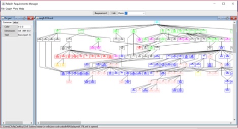
Fig. 21. Visualizing graphs of requirements in PaladinRM.
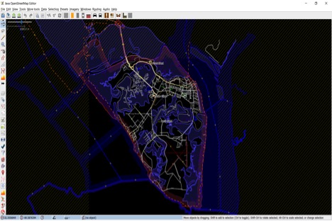
Fig. 20. U.S. Marine Corps Recruit Depot, Parris Island, South Carolina.
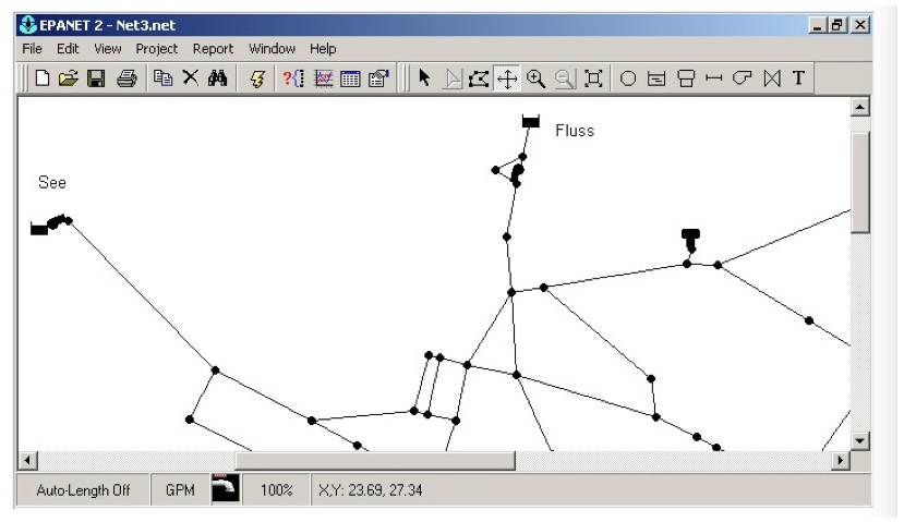
Fig. 19. Graphical display of a water distribution piping system.
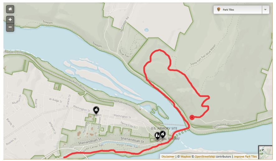
Fig. 18. Example of Highlighted Best Path Suggestion.
(Source: https://www.nps.gov/hafe/planyourvisit/maps.htm)
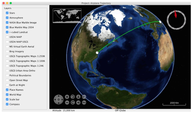
Fig. 17. Using NASA World Wind to Model and Visualize Airplane Trajectories.
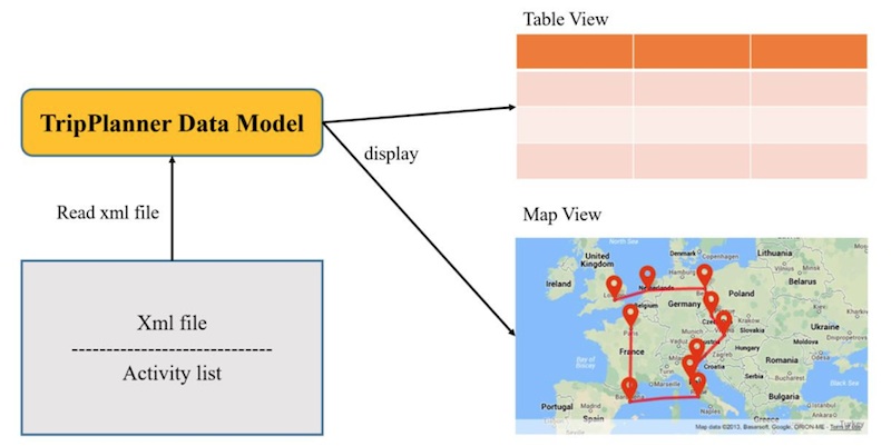
Fig. 16a. Software architecture for trip planner data model.
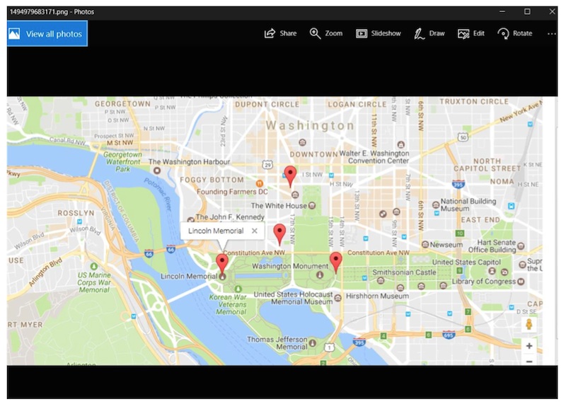
Fig. 16b. Visualization of map locations in Washington DC.
Project goal is to explore opportunities for linking Natural Language Processing with physical and geographical system domain analysis.
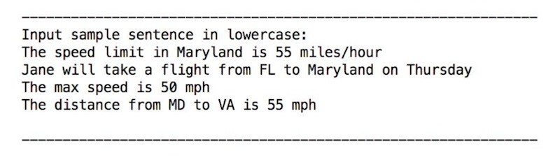
Fig. 15a. Sample sentences.
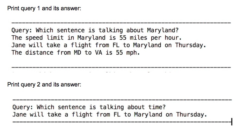
Fig. 15b. Querying sample sentences for physical and geographical content.
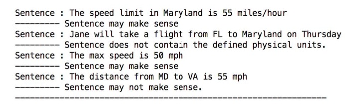
Fig. 15c. Simple tests to see if a sentence actually makes sense?
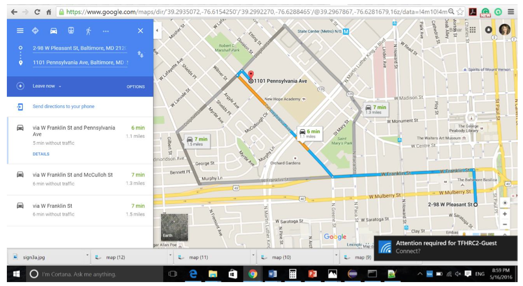
Fig. 14a. Using Google Maps to estimate travel time.
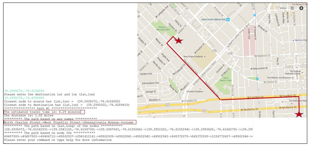
Fig. 14b. Proposed method: Modeling urban travel time with JGraphT,
a stepping stone to working with
GraphHopper .
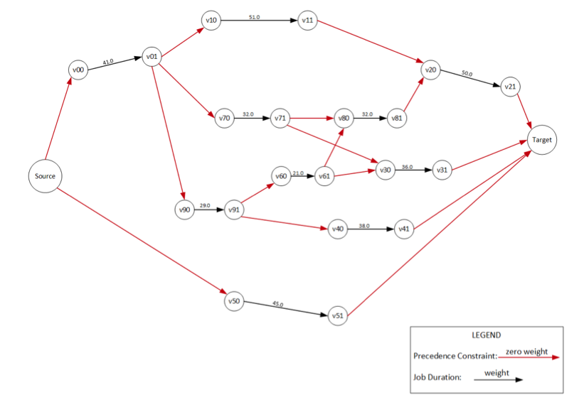
Fig. 13a. Graphical layout of jobs with precedence constraints.
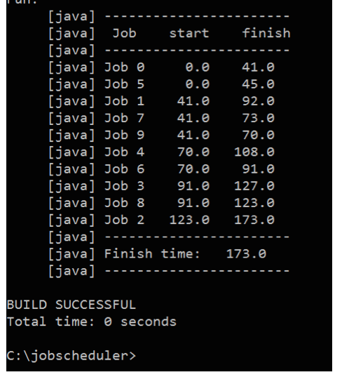
Fig. 13b. Sceendump of output from job scheduler.
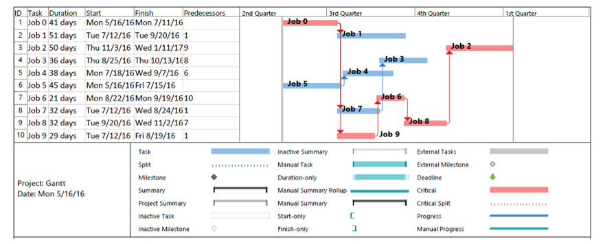
Fig. 13c. Gant chart for job scheduling problem.
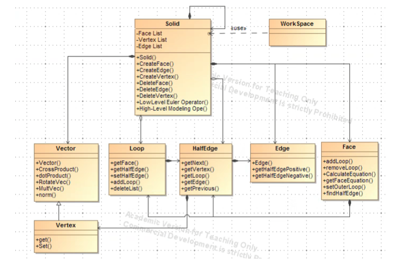
Fig. 12a. Class diagram for modeling of closed solids.
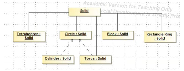
Fig. 12b. Object diagram for modeling of solids.
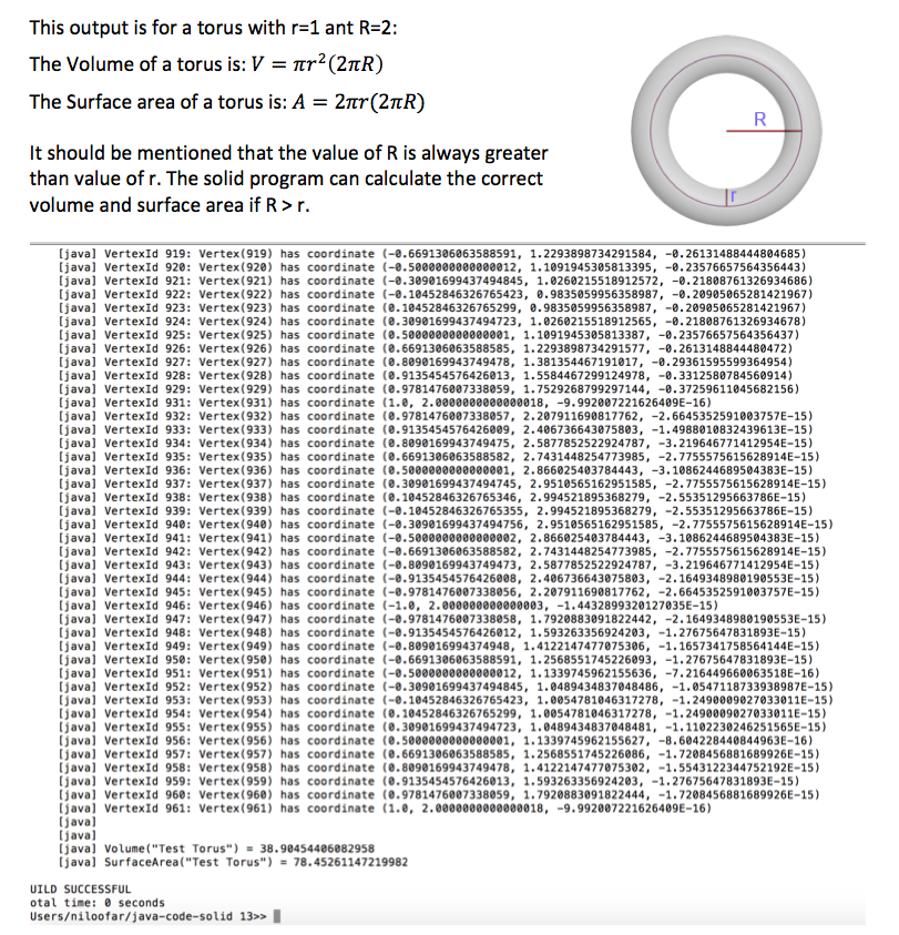
Fig. 12c. Compute surface area and volume of a torus.
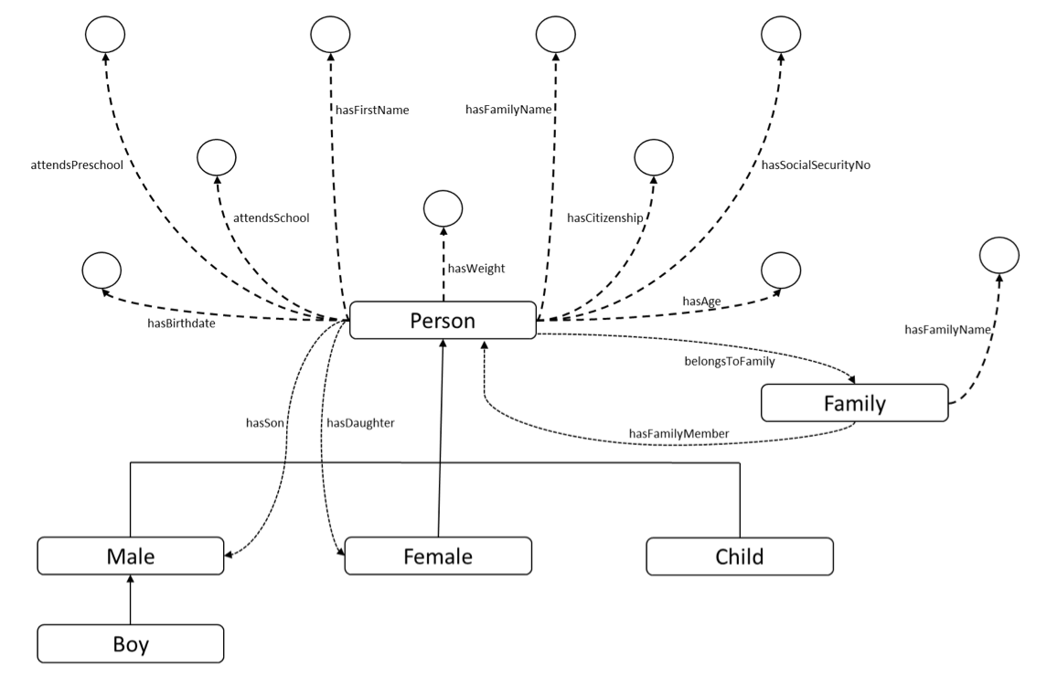
Fig. 11a. Semantic graph model for a person.
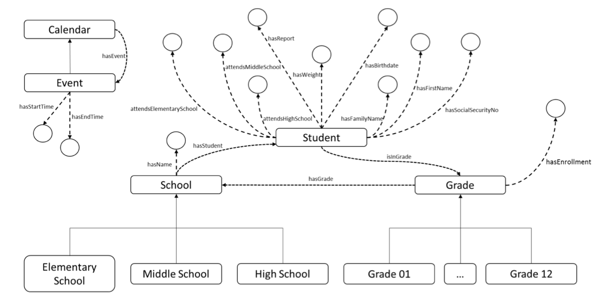
Fig. 11b. Semantic graph model for a school system.
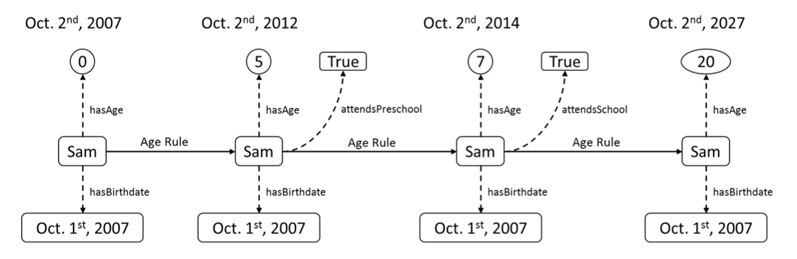
Fig. 11c. Event-based modeling of properties associated with a person.
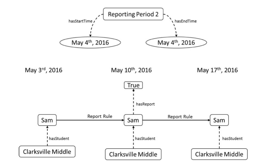
Fig. 11d. Interaction of events (intervals of time) and semantic properties for sending a school report home.
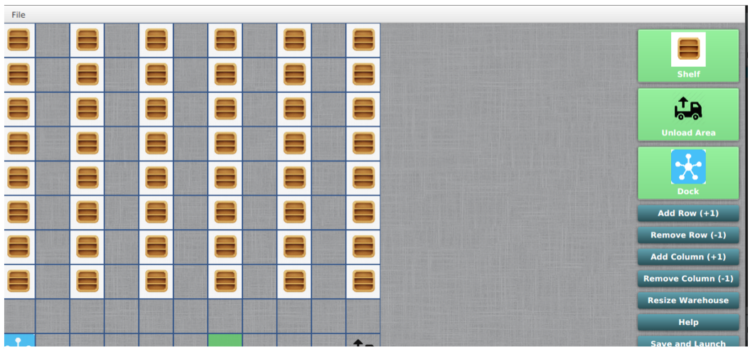
Fig. 10a. Designed warehouse layout.
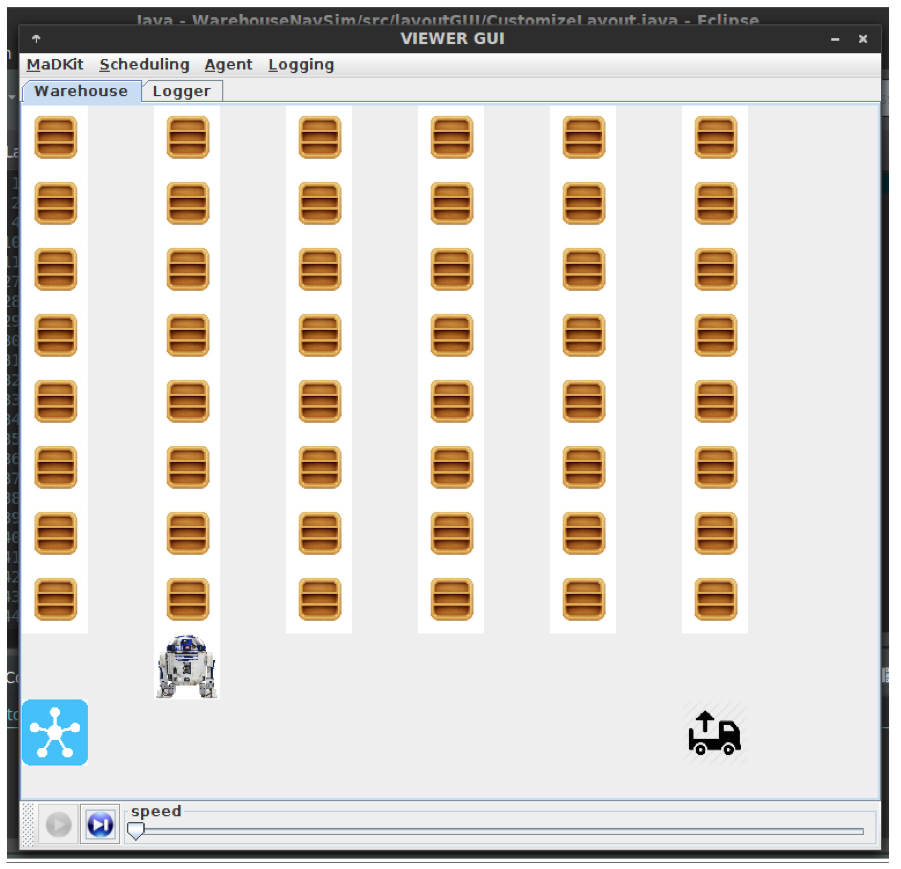
Fig. 10b. Warehouse view of running simulation.
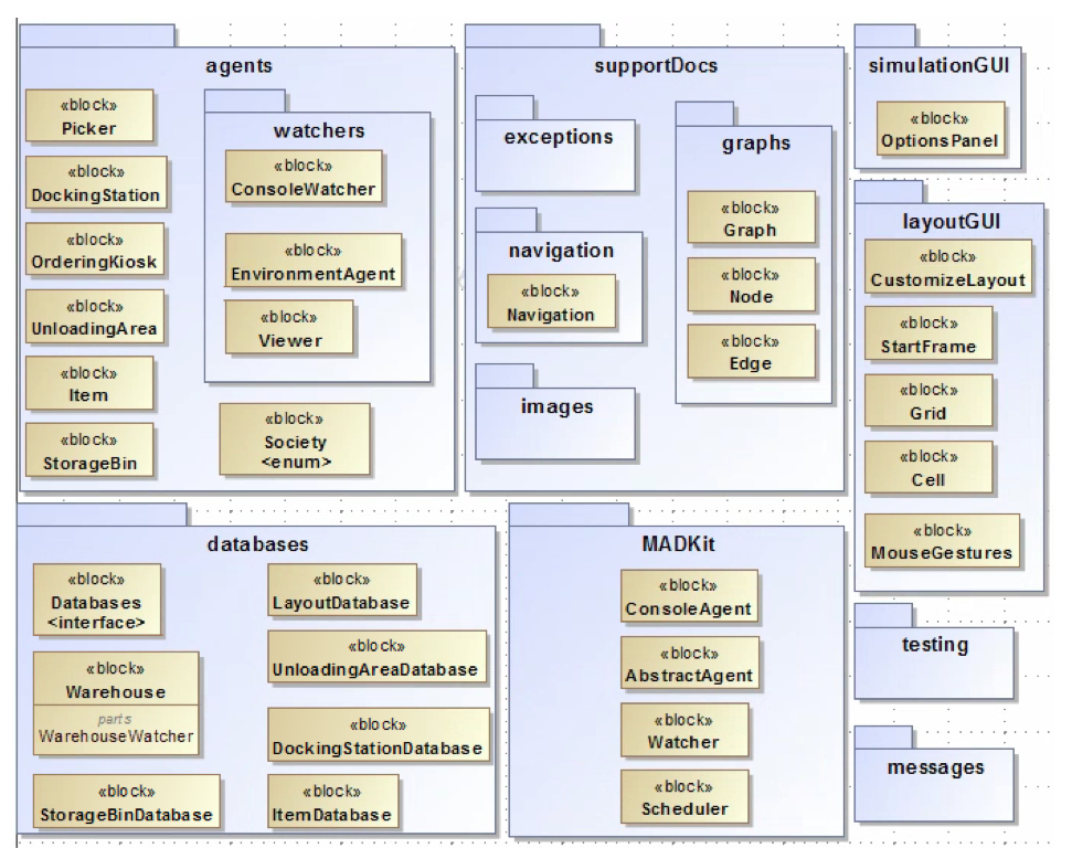
Fig. 10c. Package diagram for warehouse simulation.
Fig. 09a. Satellite view of the project area, annotated with the points of interest.
Fig. 09b. A snapshot of the route selection dataset.
Fig. 08a. Class diagram of a City Meta-Model.
Fig. 08b. Modeling cascading failures within the City System. Incipient failure.
Fig. 08c. Modeling cascading failures within the City System.
Propagation of failures across systems.
Fig. 07. Solid modeling and Java 3D visualization of a tank!
Fig. 06a. Pump connected to a pipe in a network.
Fig. 06b. Physical model of fluid flow in a pipe of length L.
Fig. 06c. Application of Bernoull's equation in pipe flow.
Fig. 06d. Pipe and pump components connected into a simple network.
Fig. 06e. Pipe 2's output pressure as a function of the pump discharge pressure.
Project 05: Dam Structure Modeling and Visualization
Author: Qianli Deng (Shally)
Semester: Spring 2012
Fig. 05. Java 3D visualization of Lac qui Parle Dam.
Project 04: Safe and Efficient Bicycle Routes
Authors: Leah Flake and Sapeksha Vemulapati
Semester: Spring 2012
Fig. 04a. Bicycle safety map (red = 5, orange = 4, yellow = 3, green = 2, blue = 1)
Fig. 04b. Weighted graph network of vertices and edges (only seen by the developer)
Fig. 04c. Display of the shortest route.
Project 03: Graph-based modeling of a People Mover Train
Author: Reuben Juster
Semester: Spring 2012
Fig. 03. Graph model of the AirTrain at JFK Airport.
Project 02: European Gas Network Modeling
Author: Jonathon Kumi
Semester: Spring 2012
Fig. 02. Movement of flows in the European Gas Network.
Project 01: Architectural Floorplan Modeling of Buildings
Authors: Eddie Tseng and Mamadou Faye
Semester: Spring 2012

Fig. 01. Composite hierarchy display of the SEIL (Systems Engineering and Integration Laboratory) floorplan.
Last Modified: January 25, 2018.