[ Project 1 ]: Bike Sharing Prediction in London
[ Project 2 ]: Fuel-Type Choice Prediction using Variational AutoEncoder
[ Project 3 ]: Classification of Structural Images using Convolution Neural Networks
[ Project 4 ]: Aircraft Activity Identification in Small General Aviation (GA) Airport
[ Project 5 ]: Estimating Air Travel Trends in the U.S. with Passively Collected Mobile
Device Location Data
[ Project 6 ]: Design Patterns for Short-Term Prediction of Energy Consumption
[ Project 7 ]: Nationwide Annual Average Daily Traffic (AADT) Estimation on
Non-Federal Aid System (NFAS)
[ Project 8 ]: COVID-19 Detection with Neural Network
[ Project 9 ]: AI for Understanding Risks in Major Transportation Projects
[ Project 10 ]: Speed Prediction in a Traffic Corridor
[ Project 11 ]: Data Mining of Motor Vehicle Accidents in NYC
Title: Bike Sharing Prediction in London
Author: Aliakbar Kabiri
Abstract: This study tends to predict the count of bike sharing requests in the capital of England, London, using multiple attributes provided in a dataset as follows: actual temperature, real feel of the temperature, humidity in percentage, wind speed in km/h, the overall condition of the weather, the season, whether the day is holiday, and also whether the day is in weekend.
The dataset contains the bike sharing information of London for the entire 2015, and 2016. In this study, we plan to predict the number of bike sharing requests by evaluating different kinds of machine learning and classification approaches such as neural network, super vector machines, naive bayes, as well as regression models including multivariate linear regressions. We will report the performance of the models and pick the best one for further predictions on the new upcoming datasets. We will also explore the dataset to address some questions such as the reasons that can cause the lower number of rents, or the best situations to rent bikes, etc. As an example, the figure below shows the number of cases of dataset with different values of bike sharing requests.
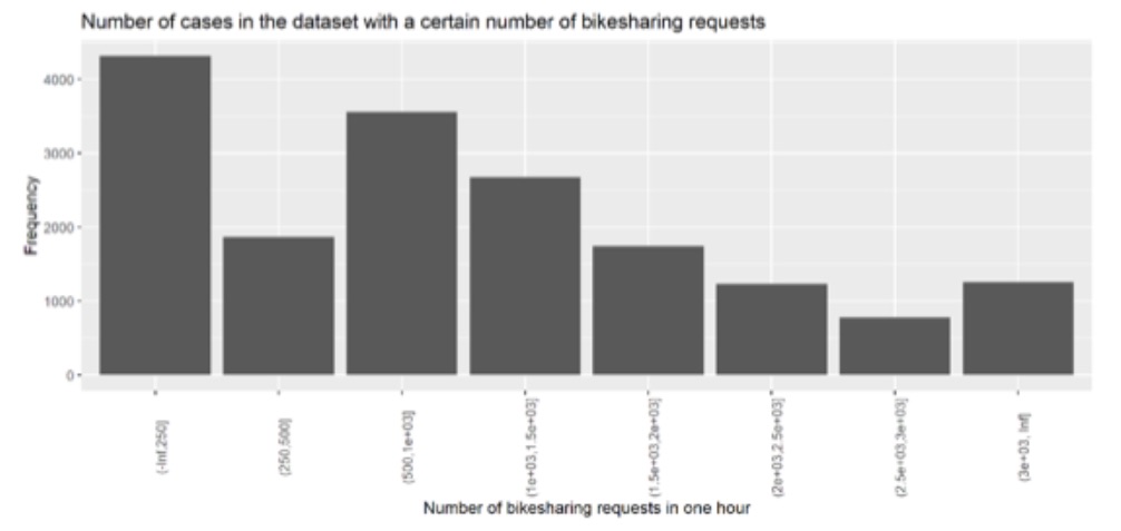
Figure 1a. Sample of bike sharing requests per hour.
Figure 1b. Categorical values in data set.
Data Sources
The data is acquired from three sources: freemeteo.com - weather data
References
Title: Fuel-Type Choice Prediction using Variational AutoEncoder
Author: Zhichao Yang
Abstract: Variational autoencoder is a technique that mainly serves to generate new observations, kind of a synthetic sample. To do so, it takes an initial real sample and through a complex process that involves two neural networks (encoder-decoder), generates new data. It is often utilized to create new images from a set of existing ones. Due to its property of reconstructing data, it can also be utilized to make prediction. The picture below shows how variational autoencoder works.
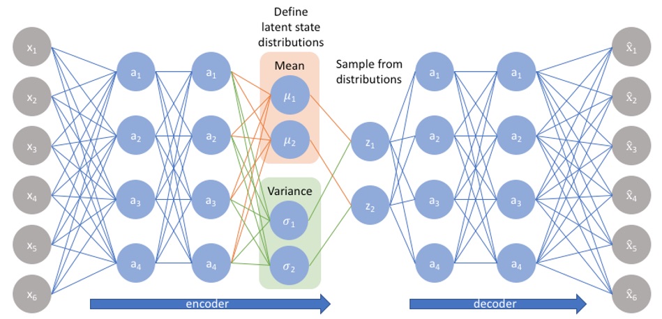
Figure 2. Network architecture for prediction of fuel-type choice.
Here, the input variables x_1,x_2,..,x_6 can be features I want to research.
Predicting future fuel type choice can help investors to hold the trend of market share of each fuel type and make reasonable decisions to invest. So make a good prediction is something important to achieve the aim. And since variational autoencoder shows promising potential in making predictions, it is a meaningful thing to take advantage of the technique. The purpose of the project is to make predictions of future fuel type choice based on current NHTS data, which is the authoritative source on the travel behavior of the American public. I will explore the feasibility and the advantages of utilizing variational autoencoder in predicting the future fuel type choice share. My long-term goal is to utilize variational autoencoder to predict more travel behavior attributes besides fuel type choice.
Data Sources
References
Title: Classification of Structural Images using Convolution Neural Networks
Author: Shivam Sharma
Abstract: With the Artificial Intelligence world getting more developed and the need of repetitive and skilled labour tasks increasing with a shortfall in the amount of skilled labour available at a moments notice for a particular task has prompted the need of machine learning models to be able to do tasks that require human level of cognition. Thankfully, with the advent of neural networks which are inspired by the human brain have become more powerful in detection and classification tasks due to the abundance of high power computing.
Figure 3a. Building damage collage.
Left: pixel-level samples, Center: component-level samples, Right: structure-level samples
The goal of this project is to classify structural images based on their level of content. For example, if a particular image is showing the entire structure, a structural object, or a small section of the object called the pixel level.
To do the above-mentioned task a convolutional neural network (CNN) was designed to classify these images based on their object level defined earlier. Each level was attached to the image with the Pixel level as 0 object level as 1 and the structure level as 2. With these labels a data set curated by the PEER HUB team was used which included approximately 30,000 images which had been individually labelled and segmented into 80% training Data and 20% testing data. The CNN will use filters to scan each image, i.e., their pixel values and develop a feature map which it uses to compare to other images and check what values match and further refine its filters by backtracking on the neural network in order to get better accuracy.
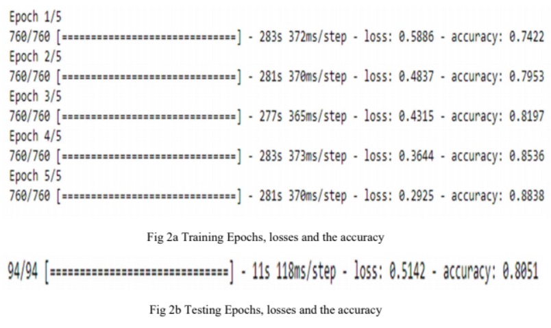
Figure 3b. Prelimininary experiments: training and testing epoch.
After putting the dataset through an Accuracy of 88% was achieved on the training dataset and an accuracy of 80% was achieved on the test dataset.
To further improve the accuracy, the architecture of the CNN needs to be changed by most probably adding more dense and convolutional layer or simply running this dataset for more epochs.
Next Steps: The Classification between the above 3 mentioned is the first task one would need to do develop a classification hierarchy of multiple interconnected Neural Networks which would classify the Structural Images.
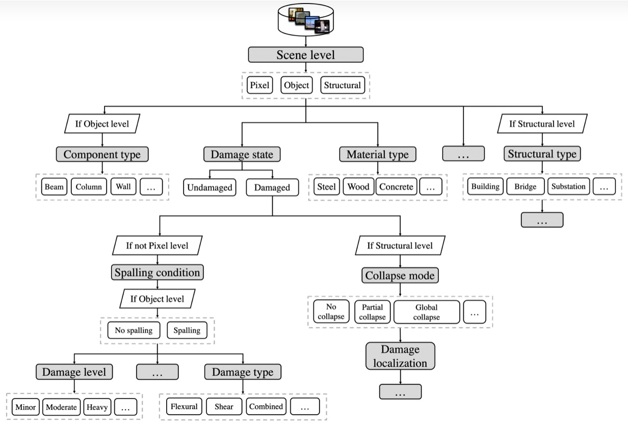
Figure 3c. Prelimininary experiments: training and testing epoch.
A longer-term roadmap that connects image classification to semantics is shown in Figure 3c.
Data Sources
References
Title: Aircraft Activity Identification in Small General Aviation (GA) Airport
Author: Danae Zoe Mitkas
Abstract: This study aims to recognize and stratify aircraft activity in a small GA airport. With ADS-B (Automatic Dependent Surveillance-Broadcast) data being widely available, either through open source databases or by installing ADS-B receivers at selected locations, extensive insight in air traffic activity has been provided to researchers. For the purpose of this study, data collected at the KOSU (Ohio State University) airport will be used. KOSU is a 3-runway airport hosting the OSU flight school, in Columbus, Ohio. The data comprises the decoded ADS-B aircraft messages, which provide a timestamp, ICAO address, latitude, longitude, altitude, groundspeed, track, rate of climb and callsign. Messages which are part of the same flight, carry the same flight_id.

Figure 4. Traffic at KOSU Airport.
The aim of this project is to identify the activity of each aircraft and to cluster it into different groups, such as arrivals, departures, touch-and-go activity or taxiing. This procedure will be a useful tool for airport managers who will be able to automatically produce accurate operation counts for each airport.
Data Sources
References
Title: Estimating Air Travel Trends in the U.S. with Passively Collected Mobile Device Location Data
Author: Mofeng Yang
Abstract: Mobile device location data (MDLD) contains abundant travel behavior information to support travel demand analysis. Compared to traditional travel surveys, MDLD has larger spatiotemporal coverage of population and its mobility. However, ground truth information such as trip origins and destinations, travel modes, and trip purposes are not included by default. Such important attributes must be imputed to maximize the usefulness of the data. This project tends to study the capability of MDLD on estimating the air travel trends. A data-driven framework is proposed to extract travel behavior information from the MDLD.
The proposed framework first identifies trip ends with a heuristic algorithm that consider the time, distance and speed between consecutive location data. Then, three types of features are extracted for each trip to impute travel modes using machine learning models. The aggregated level travel mode shares will be estimated and compared with the National Household Travel Survey at different geographies. The air travels are further filtered by considering the origin and destination distances to the nearest airport, travel time, trip distance, and aggregated by airport pairs. The air travel origin-destination flow will be validated using the airline origin and destination survey (DB1B), and the air travel attraction and production will be validated with the air carrier statistics database (T100 data bank).
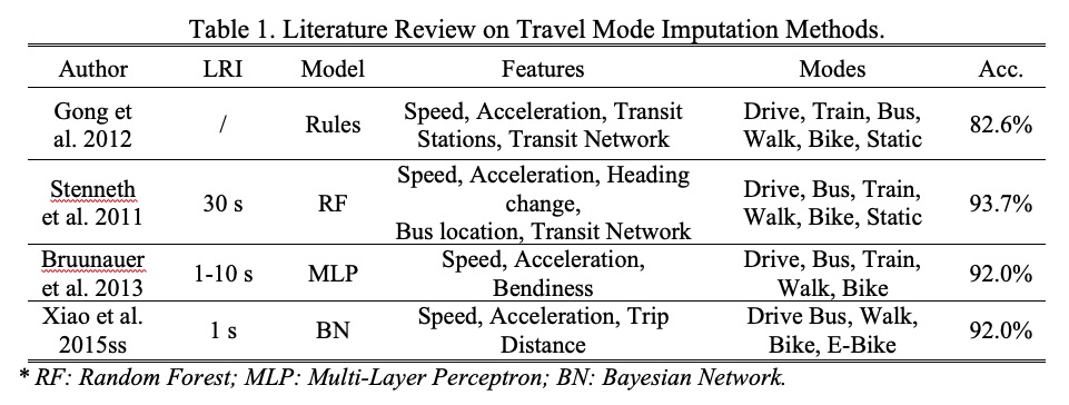
Figure 5a. Literature Review on Travel Model Imputation Methods.
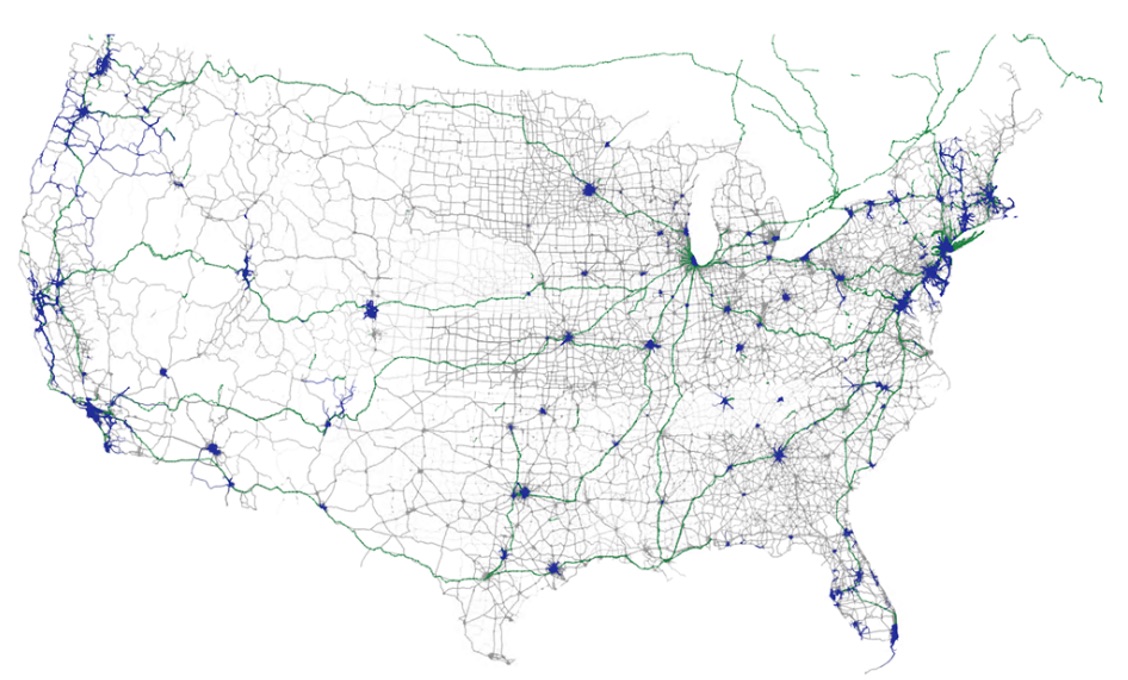
Figure 5b. Multimodal Transportation Networks: drive (grey), rail (green), rail (blue).
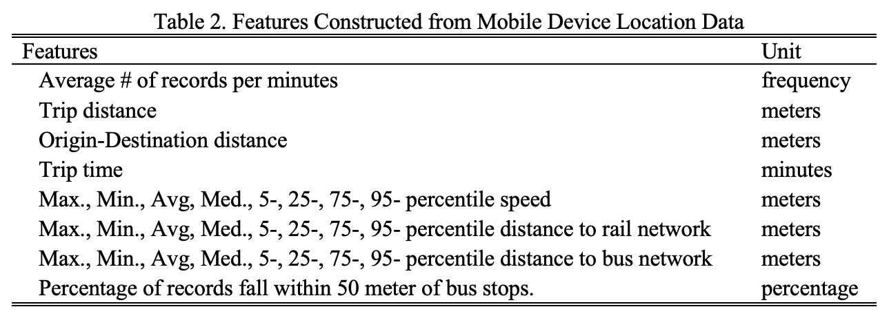
Figure 5c. Features constructed from Mobile Device Location Data.
Data Sources
incenTrip was developed by Maryland Transportation Institute (MTI) at the University of Maryland (UMD) to nudge travel behavior changes by providing real-time dynamic incentives in the Washington Metropolitan Area. incenTrip collects location data with user confirmed travel mode information, including drive, bus, rail, bike and walk.
This study uses the incenTrip app from March 2019 to January 2020 for a dedicated ground-truth MDLD data collection. During the 10-month period, fifteen designated respondents were hired to travel with incenTrip and record detailed information for each trip daily, including the start date, start time, end date, end time, origin street address, destination street address, travel time and travel mode. As a result of this data collection effort, a total number of 12688 ground-truth trip records with travel mode labels (6,064 drive trips, 1,824 rail trips, 1,403 bus trips, 1,496 bike trips and 1,901 walk trips) were obtained for the subsequent travel mode imputation model training process. The models will then be applied to the large MDLD dataset covering the entire U.S. and estimate mode shares at different geographies.
Methods
Travel mode imputation can be categorized into mainly two approaches: (1) trip-based approach; and (2) segment-based approach. The trip-based approach is based on the already identified trip ends, where each trip has only one travel mode to be imputed. The segment-based approach separates the trip into fixed-length segments (i.e., time or distance) and then impute the travel mode for each segment. Then the segment with the same travel mode will be further merged to form a single-mode trip. This study mainly considers the trip-based approach because the purpose of this study is to estimate travel mode share aggregated from individual trips.
Table 1 summarizes typical methods for travel mode imputation using the trip-based approach.
Five machine learning models, KNN, SVC, XGB, RF, and DNN are proposed to impute travel modes. The air travel modes will be further identified with heuristic rules considering the trip distance, travel time, and origin/destination distances to the nearest airport.
References
Title: Design Patterns for Short-Term Prediction of Energy Consumption
Author: Weiyi Zhou
Abstract: Predicting energy and emission consumption accurately and reliably is critical for route optimization in Eco-routing system [1-3]. One of the state-of-the-practice methods for calculating energy consumption utilizes second-by-second speed, acceleration and power demand [4]. Such models can achieve high accuracy but are not applicable for prediction purpose. Another method that can predict energy consumption uses average speed to reduce data collection and computation efforts [5]. However, it completely ignores individual driving behavior, which is particularly important in the short-term prediction of energy consumption [6].
This study aims at developing a model that exploits individual driving patterns for short-term energy prediction. The study employs long short-term memory neural network (LSTM NN) to predict the individual driving patterns using large sample floating car data. As two important inputs, average speed and volume extracted from historical traffic data. With the predicted driving pattern, a more accurate speed distribution can be used to estimate link-based energy consumption. The performance of the proposed model is evaluated by the comparison of the estimated indicators and the real values collected from in-vehicle fuel recording devices.
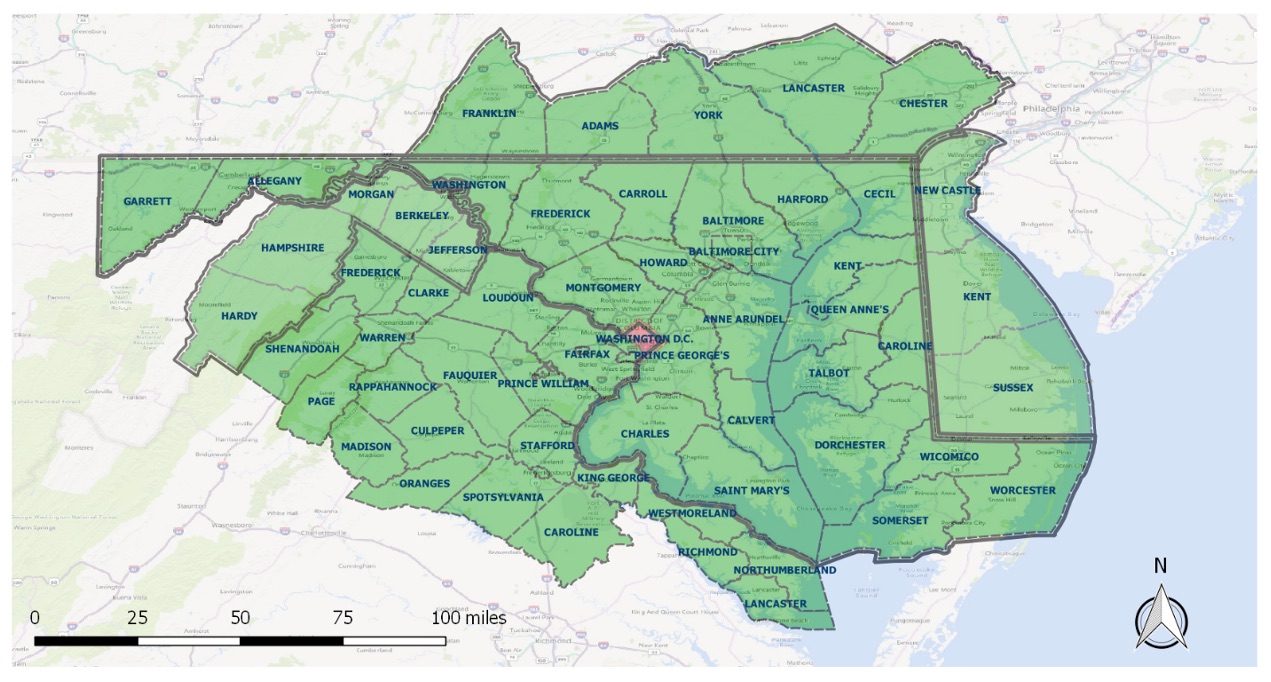
Figure 6a. Spatial coverage of i2D data.
Data Sources
The data source of this study is the naturalistic driving data collected using on-board logging system called i2D. The system consists of an on-board unit (OBU), a mobile communications network (via M2M protocols), and a secure cloud database. The OBU connects to the vehicle's OBD-II interface, and includes a GPS sensor along with a 3D accelerometer and a barometric altimeter. Multiple engine and vehicle dynamics measures are acquired from the OBU at high resolution (1 Hz). Travel information and fuel consumption are recorded in real time, and then transmitted to the online database using mobile communications.
More than 2,500 trip records at MWCOG study area (see Figure 6a) from 16 testers are collected from January 2017 to December 2018. The system stores a driver's vehicle information such as vehicle age, vehicle type, specific model, cumulated driving distance, vehicle mass, and assigned a unique user ID to the driver. Second-by-second geometry (e.g., slope, longitude and latitude), travel dynamics (e.g. speed and acceleration), energy consumption (e.g. cumulated fuel and fuel efficiency), and other information (e.g. intake air temperature (IAT), humidity, and manifold pressure (MAP)) were collected and stored in the directory under the trip ID.
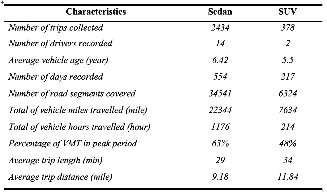
Figure 6b. Description of trip records collected from i2D data.
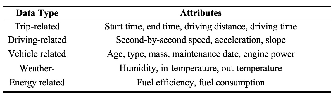
Figure 6c. Attributes of trip records in i2D data.
Trip description and the included attributes are presented in Figures 6b and 6c.
Primal Analysis
After filtering the unusable trip records, 2254 trips remain for further analysis. Figure 2-(a) ~ (d) present the distributions of travel distance, travel time, departure time, and average speed for these trips.
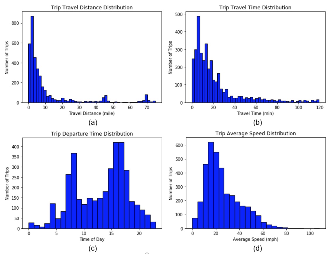
Figure 6d. Distribution of collected trips after data processing.
(a) travel distance distribution, (b) travel time distribution, (c) departure time distribution, (d) average speed distribution.
A representative example is demonstrated in Figure 3, of which the actual driving speed is significant higher than average traffic speed in most time. Yet all signs suggest that integrating driving pattern predication in short-term energy prediction is critical.
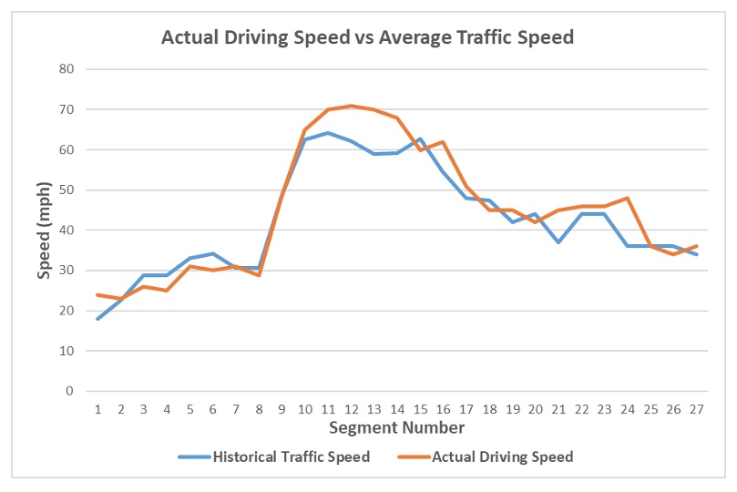
Figure 6e. Comparison of actual driving speed and average traffic speed.
References
Title: Nationwide Annual Average Daily Traffic (AADT) Estimation on Non-Federal Aid System (NFAS)
Author: Qianqian Sun
Abstract: This study aims to address the nationwide gap in Annual Average Daily Traffic (AADT) data on Non Federal Aid System roads in U.S. With a Spatial Autoregressive Model as a benchmark, two machine-learning approaches, i.e., Artificial Neural Network (Figure 7a) and Random Forest (Figure 7b), will be applied and compared in terms of the accuracy of estimating AADT according to five error measures, i.e. MSE, RSQ, RMSE, MAE, and MAPE.
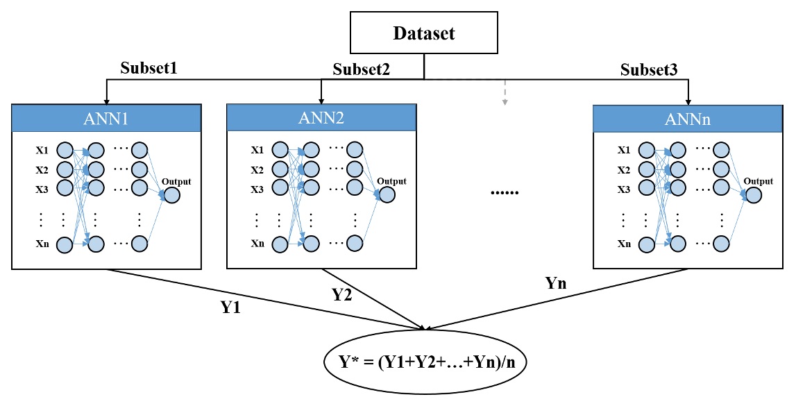
Figure 7a. Structure of ensembling artificial neural networks.
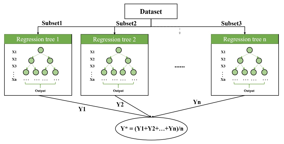
Figure 7b. Architecture of random forest.
A data-mining of the built-in environment from three perspectives, i.e., on-road and off-road features, network centralities, and neighboring influences covers 87 variables in centrality, neighboring traffic, demographics, employment, land-use diversity, road network density, urban design, and destination accessibility. Data integration using different buffering sizes and statistical analysis of linearity and monotonicity promotes the variable selection for estimation. When implementing the machine-learning approaches, not only the estimation performance will be analyzed, but also the relationship between each variable and AADT, the interplays among variables, variable importance measures will be thoroughly discussed.
Data Sources
References
Title: COVID-19 Detection with Neural Network
Author: Guangchen Zhao
Abstract: During the past several months, the SARS-COV-2 (COVID-19) pandemic has impacted mankind as a whole. Although the accuracy of the lab is above 95%, lab tests for COVID-19 take more than 24 hours. A faster way to detect COVID-19 like using chest X-ray images could speed up diagnosis and help control the spread of the COVID-19 virus. In this study, I am going to employ neural network to detect COVID-19 as well as other kinds of pneumonia.
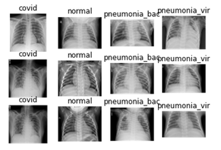
Figure 8a. Sample of 4 categories of chest x-ray.
As in a similar study posted by Yijie Xu [1], I am going to combine the Kaggle Chest X-ray dataset with the COVID-19 Chest X-ray dataset collected by Dr. Joseph Paul Cohen of the University of Montreal. Both datasets consist of posterior-anterior chest X-ray images of patients with pneumonia. The dataset has four categories, and for each category I am going to collect 200 images for study. 40 images per category are going to be used as the test set.

Figure 8b. Category and sizes of the datasets.
Data Sources
References
Title: AI for Understanding Risks in Major Transportation Projects
Author: Mazi (Abdolmajid) Erfani
Abstract: As the size and complexity of the construction projects has grown recently, much unattended, or unutilized data throughout project implementation is available. Current risk management practice heavily relies on the subject matter of expert judgment. However, a large number of major transportation projects have been completed in the last 20 years besides the advancement of artificial intelligence in various domains provide the possibility of applying machine learning and deep learning algorithms to understand risks efficiently.

Figure 9a. Abstract representation of proposed research.
This study tries to apply exciting knowledge of data mining techniques into the risk management domain to provide a better understanding of risks in the transportation projects. The study is built on a large project risk database (52 Major transportation projects including 3000 risk items) to provide following applications: Identifying the best risk category for unstructured risks (Risk classification); Automatic generation of common risks in various project specification (Risk prediction).
Data Source
Data Collection
The main source of all detailed information about the process of risk management is the risk register in transportation projects. The risk register is a 'live' document to reflect risk management practice. For this study, a dataset of risk registers including 52 major transportation projects that were completed in the last 20 years in the United States is provided.
The detailed information about the projects (Project type, Project delivery method, Project Size) is provided in the following Figure 9b.
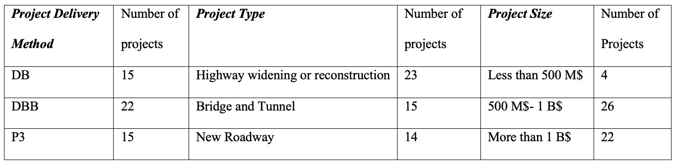
Figure 9b. Dataset from 52 transportation projects.
Overall, these 52 projects include more than 3000 risk items in which some of them are exactly similar and some are similar with different languages and terminologies. Therefore, a natural language processing approach is needed to capture the risks with the same meaning but different languages and words.
Research Design
1. Risk Classification. Numerous studies have been completed in the literature dealing with risk identification in highway and transportation projects. However, these studies may follow different risk breakdown structure and identify multiple risks. Whereas empirical transportation data show that most risk register includes a similar risk breakdown structure which can be used in general. Sometimes identified risks in the risk register are unclassified and unstructured, therefore classifying risks from unstructured format can be used to understand risks better. Among those 3121 risk items, 1345 (43%) are unclassified. On the other hand, risks classified into 10 main groups including: Construction, Contracting and Procurement, Design, Environmental and Hydraulics, Financial, Management and Organization, Right of Way, Structure and Geotechnical, Traffic Management, and Utilities and Railroads.
To classify unclassified risks into these 10 groups, it is possible to follow two different approaches:
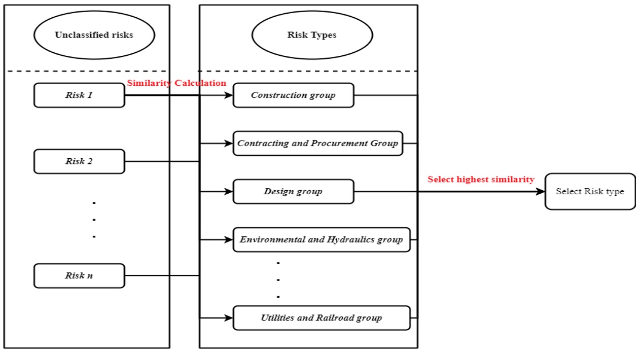
Figure 9c. Flowchart for word2vec approach to risk classification.
First, the vector that represents the new risk item should be calculated then each risk category is considered as a vector. The similarity between these two vectors which is calculated by Cosine similarity will be determine the max of similarity and risk type. To validate the model accuracy, those 1776 (47%) risk items that have a label of risk type will be used to see the model accuracy.
We can apply several classifiers provided by scikit-learn python library, including Bernoulli Naive Bayes (BNB), Support Vector Machine (SVM) with Stochastic Gradient Descent (SGD), and Logistic Regression (LR), to build the pipeline for risk classification. Vector representation can be based on TF-IDF and Word2Vec model. Therefore, classifier options will include MNB+TF-IDF, BNB+TF-IDF, SVM+TF-IDF, LR+TF-IDF, MNB+word2vec, BNB+word2vec, SVM+word2vec, LR+word2vec. The best classifier and approach will be used as the final classifier to classify the unlabeled risks.
2. Word Clouds and Top Frequent Risks. After classifying the unlabeled risks, all 3,121 risk items will be considered to find the top frequent keywords and top frequent risks in each group. The result will help the project teams to have a reliable and detailed source as a common risk register to start their risk analysis in future projects. First, a simple word cloud will be made by using the risk items to see what the top frequent keywords in each risk group are. Then, a pre-trained word2vec model will be used to match a similar risk with different terminologies. The result will be showed what are the top frequent risks in each group of risks in these 52 major transportation projects which are the most common risks.
3. Drivers Behind Similarity and Uniqueness of Risk Registers. Project type, project delivery methods, and project size are the main parameters that affect the risks and risk identification in infrastructure projects. Little is known that which factor has more impact on risk identification as well as what are the frequent risks under each project specification for major transportation projects.
In this step the similarity calculation will be at project level. All the risks in risk register one which belongs to project: (A) will match to highest similar risks from risk register two belongs to project, (B). The average of risk similarity will show how similar are the identified risks in project A and B. 52 projects in the database will be classify for each parameter (project type, project delivery method, and project size) based on Table 1 and project under each group will compare by each other. Next, a statistical analysis will be performed to compare the impact of project type, project delivery method, and project size on risk similarity at project level. Last, top frequent risks under each group of those parameters can be found like the previous step to inform project team about common risk under each project specification for transportation infrastructure projects.
4. Risk Network Analysis. As each risk register includes a multitude number of risk items, there will be an interesting question that what are the risks that usually come together. If one specific risk item is identified in one project, then the project team should consider those connected risks which have been identified in similar previous projects. This analysis will be significantly more important for top frequent risks. A network of risks will visually display the risks that are connected to top frequent risks in major transportation projects and most of the time come together. Considering the similarity of risk items with different terminologies is the basis of all steps.
5. Deep Neural Network Training So far, all the analysis is based on using a pre-trained word2vec model by Google. This model was trained on google news words to convert each word to a 300-dimension vector. Therefore, training a neural network over our data could result in better model accuracy. Training a custom word2vec model using Genism and TensorFlow based on the words in the corpus using deep learning will be the aim of this part.
Post-Course Publication of Project
Erfani A., Cui Q., and Cavanaugh I.,
An Empirical Analysis of Risk Similarity among
Major Transportation Projects using Natural Language Processing
(asce library),
Journal of Construction Engineering and Management, ASCE, Vol. 147, No. 12, December 2021.
References
Title: Speed Prediction in a Traffic Corridor
Author: Romina Jahangiri and Majed Hamed
Abstract: Traffic speed is an important indicator of congestion, incidents, and bottlenecks in traffic network. Vehicle probe data is widely used to provide (near) real-time measurements of the field speeds. Predicted speeds can be used to plan for traffic control measures and to allocate assets to problem areas.
In this project a machine learning model will be trained to estimate and predict traffic speeds on the Capital Beltway (I-495) based on archived 2019 data. Weather data can be used to predict the speed in the different weather types for future.
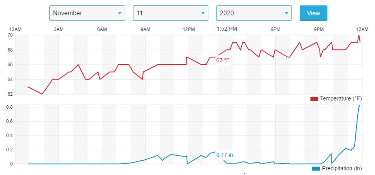
Figure 10. Temperature and precipitation vs time on Capital Beltway. Nov. 11, 2019.
Figure 10 shows, for example, the time-variation of precipitation during 11th of November, 2019. Speed data of I-495 also is available. So, with combining these two data, in this study we can predict the impact of weather on vehicles speed.
Data Sources
Title: Data Mining of Motor Vehicle Accidents in NYC
Author: Donald Dzedzy
Abstract: Motor vehicle accident data where someone is injured or killed, or where there is at least $1000 worth of damage has been captured by police reports within the boundaries of New York City over the past 5 years. This project aims to use data mining to look if any of the parameters of the data highlight an increased risk of these accidents.
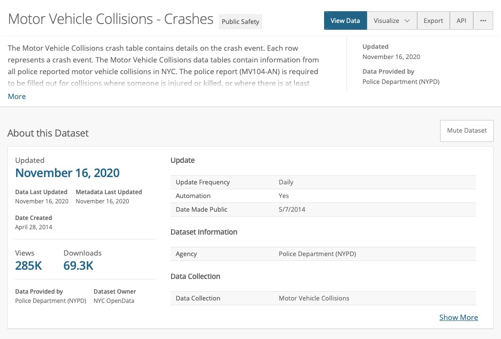
Figure 11. Dataset for motor vehicle accidents in NYC.
Thinking thus far:
There are over a million records from the past 5 years. It would appear there will need to be some data cleaning done but I figure I could look if any of the key categories from time of day, location, car type, possible cause (when listed), etc... is more significant in an accident than any other. To add to this I thought I might be able to merge in weather data (rain/cloudy sunny on a specific day), if I can find it, and see if that correlates to an increase in accidents. Another thought is if the location data is any good I could try maping it in OpenMaps. And last thought would be the ability to predict accidents in the next day/week/month given all this historical data to do a little machine learning too. I guess it all depends on how the first part goes and what else I can get to in the remainder of the semester.
Data Sources
Last Modified: November 17, 2020,
Copyright © 2020, Department of Civil and Environmental Engineering, University of Maryland.