 OPTIMIZATION OF ENGINEERING SYSTEMS TUTORIAL
Optimization is the process of obtaining the best result or benefit under a given set of circumstannces. Optimization-based approaches to design are desirable from the standpoint of providing and engineer with a formal structure for transforming an operational need into a system that will deliver a prescribed level of performance. Indeed, throughout all stages of engineering product's lifecycle, engineering and business decisions are made with the ultimate goal of maximizing/minimizing a goal or benefit while also balancing, or controling the use of, limited resources and meeting zero or more constraints.
The size and complexity of optimization problems that can be solved in a reasonable time has been advanced by the advent of modern computing technologies. Modern computing technologies have, in turn, spurred the development of new methods for solving optimization problems.
In this tutorial we will learn how to formulate linear and nonlinear optimization problems, and compute their solutions using the MATLAB Optimization Toolbox and CPLEX. This tutorial an introduction in the sense that only the most basic optimization concepts and algorithms are explained in depth.
Engineering Applications of Optimization
Within the traditional engineering disciplines, optimization techniques are commonly employed for a variety of problems, including:
Of course there are many variations on these themes. Optimization problems can be formulated in terms of economic returns relative to resources invested. Some optimization problem have multiple objectives -- the values of these objectives need to be balanced while also satisfying the problem constraints.
Systems Engineering View of Optimization
The systems engineering view of optimization
encompasses the abovementioned applications,
but goes the extra step of explicitly attempting
to apply optimization at those stages of the product lifecycle
having the greatest opportunity for improvement.

Figure 1 shows two streams of information. The heavy solid lines show how funds committed and funds expended vary throughout the product lifecycle. The gap between these contours is greatest during the conceptual stages of design.
The second stream of information shows how our knowledge of a system changes during the product lifecycle, and how easy changes are to fix. The good news is that even though our knowledge of a system is incomplete in the beginning, changes are cheap to make. The bad news is that once key decisions have been fixed in place, large sums of money are committed for the remainder of the project. Hence the quality of decision making in the early stages of the product lifecyle is of utmost importance.
Part of the problem can be solved with a thorough gathering of requirements...once this information is in hand, one still needs to make the best decision possible. The latter can be accomplished through the use of engineering models (to learn about system behavior) and optimization techniques (for guidance on the best way to change a system for potential improvements).
In systems engineering terminology, the ``effectiveness measures'' are those aspects of a problem that will participate in either the system optimization and/or trade-off studies. There are usually multiple measures of system effectiveness. Allocated requirements place constraints on the design process. Hence, an optimal system design is a constrained optimization problem.
MATHEMATICAL PROBLEM STATEMENT
In this section we describe a step-by-step procedure for creating optimization models, and then describe the features of unconstrained and constrained problems.
Formulation of Optimization Models
The step-by-step procedure for formulating an optimization model is as follows:
As we will soon see, the design constraints and design objectives can sometimes be expresses as mathematical functions of the decision variables.
Unconstrained Optimization Problem
We wish to find an n-dimensional design vector
X = [ x_1, x_2, x_3, ..... x_n ]
that will minimize (or maximize) a functional objective
Objective = f(X).
If f(x) is differentiable, compute the gradient of f, set it equal to zero, and solve for the values of "x" that minimize f(x).
Check that the solution is a minumum by computing the (Hessian)
second derivative of f(x). A mimimum point will
be indicated by a positive sign on the Hessian.
See, for example, the left-hand side of Figure 2.

The right-hand side of Figure 2 shows a variety of ways in which the task of finding a solution can become difficult. Sources of difficulty include multiple minima, regions of degenerate minima, points that are nondifferentiable, and regions where the function simply is not defined.
Constrained Optimization Problem
We wish to find an n-dimensional design vector
X = [ x_1, x_2, x_3, ..... x_n ]
that will minimize (or maximize) a functional objective
Objective = f(X).
In many optimization problems the space of permissible design vectors is not entirely free, but bounded by a family of constraints. For example, constraints naturally arise from upper bounds on limited resources, physical quantities that must be greater/less than zero for a problem to make sense, and so forth.
From a mathematical standpoint, constraints fall in to three broad categories. Inequality constraints (also called conventional constraints) are of the form:
G_i (x) <= 0 for i = 1, 2, ... m.
Equality constraints are of the form:
E_j (x) = 0 for j = 1, 2, ... p.
Functional constraints are of the form:
    F_k (x,t) <= 0     for    k = 1, 2, ... q.
                       and    t_min <= t <= t_max.
The total number of constraints is m+p+q, and for optimization problems modeling real-world applications, can easily number into the thousands.
In a constrained optimization problem, the search space of possible solutions is restricted by convenctional and functional constraints. Solutions are found by combining the constraints with the objective function(s), and then choosing an appropriate search algorithm.
SEARCH METHODS
Once a mathematical programming problem has been classified, we need to find a solution using an appropriate search method. That is, a course of action for seeking a solution to the optimization problem that has been posed. Four types of search method are common:
For some simple problems, an optimal solution may be obtainable directly. Otherwise, the standard technique for solving optimization problems is to compute a sequence of solutions to simplified approximations of the original problem. The iterative procedure stops when no improvement is possible.
Calculus-based optimization methods are useful for finding the minumum value(s) of functions that are continuous and differentiable. They employ sensitivity information to form local models of a larger problem. The purpose of the local models is to approximate the true objective function and constraint functions, thereby providing a direction of change for improving the design. A solution to the larger optimization problem is computed via a sequence of updates provided by the local models. The search procedure is terminated when the sensitivity information indicates a local minima has been reached.
This class of problems is important because they form the basis of many much more sophisticated techniques for optimization-based engineering design.
MATHEMATICAL CONCEPTS
Techniques for computing the minumum/maximum values of functions draw on the following concepts:
Convexity of functions
Definition. Let f be a function from R^n onto R, and X be a subset of R^n. The function f is convex if
f( a*X + (1-a)*Y ) <= a*f(X) + (1-a)*f(Y)
See Figure 3.

Local Minimum of Functions.
Set Constraints. Consider the problem
min f(x),
subject to x inside the convex set X element of R^n. Let grad f be the gradient of f. The point x* is a local minimum of f over X if
{grad f(x*)}^T . (x - x*) >= 0
for all x in X.
Global Minumum of Functions. A vector x* is a global minumum of a convex function f over a convex set X element of R^n if and only if:
{grad f (x*)}^T . (x - x*) >= 0
Extreme Point. If f(x) has an extreme point (maximum or minumum) at x = x* and if the first partial derivatives of f(x) exist at x*, then
{df/dx_1}(x*) = {df/dx_2}(x*) = ... = {df/dx_n}(x*) = 0.
A sufficient condition for a stationary point x* to be an extreme point is that the matrix of second partial derivatives (also called the Hessian matrix) of f(x) evaluated at x* is: (1) positive definite when x* is a minumum point, and (2) negative definite when x* is a maximum point.
UNCONSTRAINED OPTIMIZATION PROBLEMS
Add content soon .... on method of steepest descent....
CONSTRAINED OPTIMIZATION PROBLEMS
Add content soon ....
Method of Lagrange Multipliers
Add content soon ....
What is Linear Programing?
The standard form of a linear programming problem with m constraints and n variables is as follows:
    Mimimize (or Maximize) Z = c_1 * x_1 + c_2 * x_2 + .... + c_n * x_n

    Subject to:

        a_11 * x_1 + a_12 * x_2 + ... + a_1n * x_n = b_1
        a_21 * x_1 + a_22 * x_2 + ... + a_2n * x_n = b_2

        .....

        a_m1 * x_1 + a_m2 * x_2 + ... + a_mn * x_n = b_m

                   x_1 >= 0; x_2 >= 0;  ..... x_n >= 0.
                   b_1 >= 0; b_2 >= 0;  ..... b_m >= 0.
The key feature of this formulation are:
Matrix Notation
In matrix form, the standard linear programming problem is:
    Minimize (or maximise) Z = C.X

    Subject to A.X = B, X >= 0, and B >= 0.
Here, C is a 1-by-n row vector for the system cost, A is a m-by-n coefficient matrix, X is a n-by-1 decision vector, and B is a m-by-1 requirement/constraint vector.
Example. Suppose that we want to maximize
Z = 5.x_1 + 2.x_2 + 3.x_3 - x_4 + x_5;
subject to
      x_1 + 2.x_2 + 2.x_3 - x_4        = 8;
    3.x_1 + 4.x_2 +   x_3       + x_5  = 7;
and
x_1 >= 0, x_2 >= 0, x_3 >= 0, x_4 >= 0, and x_5 >= 0.
The matrix formulation of this problem is:
    Z = C.X
    where

        C = [ 5 2 3 -1 1 ];
    and
        X = [ x_1, x_2, x_3, x_4, x_5 ]^T
The constraint matrices are
     A = [ 1 2 2 1 0 ]
         [ 3 4 1 0 1 ]

and  B = [ 8 ]
         [ 7 ]
HANDLING INEQUALITY CONSTRAINTS
A linear constraint
sum_{i=j to N} a_ij . x_j <= b_i
can be converted to an equality constraint by adding a new nonnegative variable to the left-hand side of the inequality. The new variable will have a numerical value equal to the difference of the right-hand side minus the left-hand side. This so-called slack variable represents the waste involved in that phase of the system by the constraint.
Example. Suppose that we wish to maximize
Objective = 10*x_1 + 11*x_2
Subject to the constraint pair:
     5*x_1 + 4*x_2 <= 40
     2*x_1 + 4*x_2 <= 24
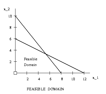
and x_1 >= 0 and x_2 >= 0. Together these four
constraints define the feasible domain shown in Figure 4.
We can convert the constraint pair to equality constraints by adding two slackness variables, namely:
    5*x_1 + 4*x_2 + x_3       = 40
    2*x_1 + 4*x_2       + x_4 = 24
and enforcing x_1 >= 0, x_2 >= 0, x_3 >= 0 and x_4 >= 0.
The matrix formulation of this problem is:
    Z = C.X
    where

        C = [ -10 -11  0  0 ];
    and
        X = [ x_1, x_2, x_3, x_4, ]^T
Notice how we have changed the maximize problem to a minimize problem by changing the sign on the objective function coefficients. The constraint matrices are
     A = [ 5 4 1 0 ]
         [ 2 4 0 1 ]

and  B = [ 40 ]
         [ 24 ]
In the following sections, we present solutions to this problem using graphics and MATLAB.
MATHEMATICAL CONCEPTS
Convex Sets
Definition. A set X belonging to R^n is convex if for every x and y in X and all values of a, 0 <= a <= 1,
a * x + (1-a) * y
is in X. In otherwords, a set is convex if the entire line
lies within X, as shown in Figure 5.

Extreme Point Solutions
A vector P is an extreme point of a convex set if it cannot be expressed as a convex combination of two other vectors in the set. That is, an extreme point does not lie on the line segement between any other two vectors in the set.
Theorem. The solution space of a set of simultaneous linear equations is a convex set having a finite number of extreme points.
Set of Feasible Solutions. Let P designate the set of all vectors that satisfy
A*X = B and X >= 0.
From the previous theorem and from the fact that convex sets interset in convex sets, P is a convex set having a finite number of extreme point solutions.
Optimal Solution(s).
If matrix A has m rows and n columns, with m <= n, then the extreme points of P have at least n-m zero components.
For a closed set of possible solutions,
the objective function attains its optimum
value (either maximum or minimum) at an extreme point of P.
The optimal solution will lie at either a unique point (i.e.,
at a corner of the search space), or along a surface.
Solutions of the latter type are called degenerate.

Consider, for example, the arrangement of constraints and objective function contours shown in Figure 4. The arrow shows the direction of increasing objective function. Since constraint 3 is parallel to the contours of constant ojective function, any solution that we choose along constraint 3, which also lies between constraints 1 and 4, is optimum.
A number of computationally efficient algorithms have been devised for the calculation of unique solutions (when they exist).
Unbounded Feasible Domain
Figure 5 shows a scenario where the feasible domain is unbounded.
The arrow shows the direction of increasing objective function value.
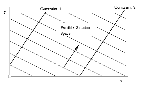
Even though the feasible domain is unbounded, a solution to the minumum objective function exists (it lies at the origin). However, a maximum value for the objective function does not exist.
CORNER-POINT SOLUTION METHODS
Theoretical considerations in linear optimization indicate that an optimal solution to any problem will lie at a corner point (or extreme point) within the feasible domain.
Hence, in the corner-point solution method, we find the optimal solution by systematically evaluating the objective function at all of the corner points in the feasible design space.
Example.
Figure 6 shows the feasible domain of the aforementioned problem
together with the objective function evaluated at a corner point.

For this small problem we can compute the optimum solution by systematically evaluating the objective function at all of the corner points. Beginning at the orgin and traversing the feasible domain in a clockwise direction gives:
    Point        Coordinate (x_1, x_2)       Objective (x_1, x_2)
    -------------------------------------------------------------
        1                     ( 0, 0 )                        0.0
        2                     ( 0, 6 )                       66.0
        3             ( 5 1/3, 3 1/3 )                       90.0
        4                     ( 8, 0 )                       80.0
    -------------------------------------------------------------
Hence, we see that within the feasible domain the objective function has a minimum value of zero at point 1, and a maximum value of 90.0 at point 3.
We will validate this solution via MATLAB in just a moment.
Preliminary Assumptions
How do I access Matlab?
MATLAB can be accessed from anywhere on the Glue System (you do not need an ISR account to run MATLAB). First, type
    kiwi:~: tap matlab
    ----------------------------------------------------------------------
    Wed Aug  5 09:09:53 EDT 1998
        This is the newest version of matlab.  This version will not work
        on Digital Unix 3.2 machines.
    ----------------------------------------------------------------------
    kiwi:~:
MATLAB can be started by typing:
    kiwi:~: matlab

                            < M A T L A B (R) >
                (c) Copyright 1984-98 The MathWorks, Inc.
                            All Rights Reserved
                            Version 5.2.0.3084
                                Jan 17 1998

      To get started, type one of these: helpwin, helpdesk, or demo.
      For product information, type tour or visit www.mathworks.com.

    >>
A small MATLAB 5 graphics window will appear for a few seconds, followed by the program announcement, and the MATLAB prompt.
>>
We are now ready to start solving problems.
MATLAB Program Development with M-files
MATLAB statements can be prepared with any editor, and stored in a file for later use. Such a file is referred to as a script, or an "m-file" (since they must have a name extension of the form filename.m). Writing m-files will enhance your problem solving productivity. Suppose that we create a program file
myfile.m
in the MATLAB language. The commands in this file can be exectued by simply giving the command
myfile
from MATLAB. The MATLAB statements will run like any other MATLAB function. You do not need to compile the program since MATLAB is an interpretative (not compiled) language.
What kinds of problems can I solve using the MATLAB Optimization Toolbox?
Optimization concerns the minimization or maximization of functions. It is used to solve complex design problems in order to improve cost, reliability, and performance in a wide range of applications. The MATLAB Optimization Toolbox contains routines that implement the most widely used methods for performing minimization or maximization on general nonlinear functions. Additional routines are provided for linear programming, quadratic programming, nonlinear least squares, and solving nonlinear equations. Combined, these routines provide a comprehensive set of tools for performing optimization.
The scope of this tutorial is limited to linear programming problems, quadratic programming problems, and constrained nonlinear minimization.
MATLAB OPTIMIZATION TOOLBOX
The linear programming capablities of the MATLAB Optimization Toolbox are as follows:
solves the linear programming problem:
      minimize  f'X subject to:  Ax <= b
          X
Here, X is a n-by-one matrix of design variables, and f is a one-by-n matrix of objective function coefficients.
defines a set of lower and upper bounds on the design variables, X, so that the solution is always in the range
VLB <= X <= VUB.
sets the initial starting point to X0.
indicates that the first N constraints defined by A and b are equality constraints.
controls the level of warning messages displayed. Warning messages can be turned off DISPLAY = -1.
returns the set of Lagrangian multipliers, LAMBDA, at the solution.
also returns a string how that indicates error conditions at the final iteration.
LP produces warning messages when the solution is either unbounded or infeasible.
EXAMPLES : LINEAR PROGRAMMING
Here I would like to provide you a brief example showing how linear programing would be applied in our daily life. You also can solve many engineering problems by mathematical way instead by your emotion. When you become familiar with it, you not only can optimize the performace of the system but also can evaluate the performace of the systems by linear programing. Now let us begin from the ground.
Example 1 : Simple Mathematical Programming Problem.
Objective Function
max : 29 * x1 + 45 * x2
Constraints
    2 * x1 + 8 * x2 <=60
    4 * x1 + 4 * x2 <= 60
        x1          >=0
                 x2 >=0
We transform it to following matrix format, than we can use lp function to do optimization
A * X <= B
where
     A =  [ 2    8;

            4    4;

           -1    0;

            0   -1];

     X = [ x1, x2, x3];
     B = [ 60; 60; 0; 0];
we also transform the objective function to
    [ 29, 45 ] * [x1
                  x2]
Now we can use MATLAB lp function to get the optimal solution, the M-File code is as follows
    M = [ 2  8 ;
          4  4 ;
         -1  0 ;
          0 -1 ];

    V = [ 60 60 0 0 ];
    v = reshape (V,4,1);
    C = [-29 -45];
    c = reshape(C,2,1);
    X0  = zeros (1,2);
    x0  = reshape (X0, 2, 1);
    xlo = zeros(2,1);
    xhi = [];
    n = 0;

    [ x, lambda, how] = lp(c, M, v, xlo, xhi, X0, n);

    how
    x
    obj = c' * x
    con = M*x - v
and the output would be like this
    x =
        10.0000
         5.0000
    obj =
           -515
    con =
        -0.0000
              0
       -10.0000
        -5.0000
now I want to show you what it means in a real x-y plane. Notice blue line
stands for constraint and red line stands for objective function.

Here is the MATLAB code for Figure 6.
    x = [ -5: 1.: 40.0 ];

    y1 = 7.5 - 0.25 * x
    plot(x,y)
    hold on

    x  = [-5: 1.: 40];
    y1 = 15 - x
    plot(x,y1)
    hold on

    x  = [-5: 1.: 40];
    y2 = 11.44 - 0.644 * x
    plot(x,y2,'r')
    hold on

    axis( [ 0, 40, 0, 20 ] )

    xlabel('X');
    ylabel('Y');
Example 2 : Simple Mathematical Programming Problem.
The same as Ex1-1, I try to change my constraint to the objective function and you will notice the difference after that. Red words stands for changings.
Objective function
max : 29 * x1 + 45 * x2
Constraints
    2 * x1 + 8 * x2 <=40
    4 * x1 + 4 * x2 <=80
        x1          >=0
                 x2 >=0
We transform it to following matrix format, than we can use lp function to do optimization
A * X <= B
where
    A =  [ 2    8;
           4    4;
          -1    0;
           0   -1];

    X = [ x1, x2, x3];
    B = [ 40; 80; 0; 0];
we also transform the objective function to
    [ 29, 45 ] * [x1
                  x2]
Now the M-File is
    M = [ 2  8 ;
          4  4 ;
         -1  0 ;
          0 -1 ];

    V = [ 40 80 0 0 ];

    v  = reshape (V,4,1);
    C  = [ -29  -45];
    c  = reshape(C,2,1);
    X0 = zeros (1,2);
    x0 = reshape (X0, 2, 1);
    xlo = zeros(2,1);
    xhi = [];
    n = 0;

    [ x, lambda, how] = lp(c, M, v, xlo, xhi, X0, n);

    how
    x
    obj = c' * x
    con = M*x - v
and the solution will be change too
    >>

    how = ok
    x =

         20.0000
          0.0000

    obj =

       -580.0000

    con =

         -0.0000
         -0.0000
        -20.0000
               0

    >>
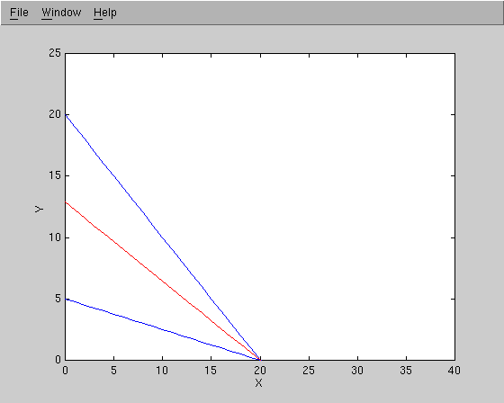
want to see the graphical interpretation? here it is! Notice blue line
stands for constraint and red line stands for objective function.
    x = [-5: 1.: 40];
    y = 5 - 0.25 * x;

    plot(x,y)
    hold on

    x  = [-5: 1.: 40];
    y1 = 20 -  x ;
    plot(x,y1)
    hold on

    x = [-5: 1.: 40];
    y2 = 12.88 - 0.644 * x;
    plot(x,y2,'r')
    hold on

    axis( [ 0, 40, 0, 25 ] )

    xlabel('X');
    ylabel('Y');
Example 3 : Optimal Design of Turbojet Engine.
Assume we want to build a next generation car that will be powered by 3 turbojet engine. The power of each engine is labeled as x1, x2, and x3. The total power of this car is:
x1 + 2*x2 + x3
For some engineering reasons, they are some constraints that must be considered when you decide the engine power. They are:
    2 * x1 + x2 -     x3  < =  2
   -2 * x1 + x2 - 5 * x3  > = -6
    4 * x1 + x2 +     x3  < =  6
Now we want to decide the power of each engine by linear programing. You have 2 software (Matlab, Cplex) provided in class to solve this problem.
Input file. Now we can translate the problem to the format of linear programing and then do it with MATLAB to solve the problem.
Objective function
Maximise x1 + 2 * x2 + x3 . ..... (1)
Subject to
    2 * x1 + x2 -     x3 < =  2        ..... (2)
   -2 * x1 + x2 - 5 * x3 >  = -6        ..... (3)
    4 * x1 + x2     + x3 < =  6        ..... (4)
The engine power cannot be negative, so
    x1 >= 0 ..... (5)
    x2 >= 0 ..... (6)
    x3 >= 0 ..... (7)
To make sure all equations are of the form A*X <= B, we rewrite the equations:
Equation         New Format
---------------------------------------------------
     (1)         Min    - x1 - 2 *x2 - x3
     (3)         2 * x1 - x2 + 5 * x3 <=6
     (5)         - x1 <= 0
     {6)         - x2 <= 0
     (7)         - x3 <= 0
---------------------------------------------------
Now I can present the all equations as
min    - x1 - 2 *x2 - x3

st   2 * x1 + x2 -     x3 <=  2
    -2 * x1 + x2 - 5 * x3 >= -6
     4 * x1 + x2 + x3     <=  6
       - x1               <= 0
       - x2               <= 0
       - x3               <= 0
In matrix form the constraint relationships may be written:
A * X <= B
where
    A  =  [  2  -1   1;
             4   1   1;
             2  -1   5;
            -1   0   0;
             0  -1   0;
             0   0  -1  ];

    X  =  [ x1;  x2;  x3 ];

    B  =  [ 12;  6;  6;  0;  0;  0 ];
also transform the objective function to
                   [ x1
     [ -1 -2 -1] *   x2
                     x3 ]
Objective:
min C * x
subject to
M * x <= V
Here is the MATLAB code needed to solve the linear proagramming problem.
    M = [ 2  1 -1 ;
          4  1  1 ;
          2 -1  5 ;
         -1  0  0 ;
          0 -1  0 ;
          0  0 -1 ];

    V = [2 6 6 0 0 0];

    v = reshape (V,6,1);
    C = [-1 -2 -1];
    c = reshape(C,3,1);
    X0 = zeros (1,3);
    x0 = reshape (X0, 3, 1);
    xlo = zeros(3,1);
    xhi = [];
    n = 0;
    [ x, lambda, how] = lp(c, M, v, xlo, xhi, X0, n);
    how
    x
    obj = c' * x
    con = M*x - v
Running the Program
I save this file as "exp1.m", it is a MATLAB scripture file, so now I don't need to repeat all command and input data but just run it by entering filename after MATLAB prompt.
einstein:~/matlab: tap matlab
Fill in details of MATLAB program output here !!
Graphical Interpretation of Results
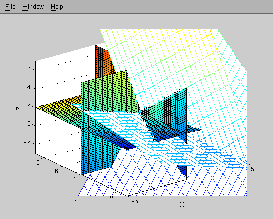
After calculation, the decision variables have come up.
    engine 1 ( x1 ) is 0.0
    engine 2 ( x2 ) is 4.0
    engine 3 ( x3 ) is 2.0
and the total power output is 10.
A plot of the constraints can be prepared with the MATLAB commands:
    x= -5:0.5:5;
    y= -5:0.5:5;
    [ X, Y] = meshgrid(x,y);

    Z1 = 2 * X + Y - 2;               % Constraint 1
    mesh( X, Y, Z1)
    hold on

    Z2 = -0.4 * X + 0.2 * Y + 1.2;    % Constraint 2
    mesh( X, Y, Z2)
    hold on

    Z3 = -4 * X - Y + 6;              % Constraint 3
    mesh( X, Y ,Z3)
    hold on

    axis([ -5, 5, -1, 9, -3, 7])
    xlabel('X')
    ylabel('Y')
    zlabel('Z')
    hold on

    x = [ -5: 0.2 : 5];
    y = [ -1: 0.2 : 9];
    z = [ -3: 0.2 : 7];
    [X,Y,Z] = meshgrid(x,y,z);

    V = X + 2 * Y + Z;
    V = real(V);
    Sx = [ 0 ];
    Sy = [ 4 ];
    Sz = [ 2 ];

    plot3(0, 4, 2,'b*')
    slice(X,Y,Z,V,Sx,Sy,Sz)    % OPTIMAL SOLUTION
What kinds of Optimization problems can CPLEX solve?
CPLEX is a tool for solving linear optimization problems, including constrained and unconstrained. Linear programming is used extensively in a wide variety of industries for solving mission-critical resource allocation problems. Examples include manufacturing scheduling, airline routing, raw material blending, financial portfolio optimization, personnel scheduling, and transportation logistics.
How do I access CPLEX?
CPLEX is only available from the Systems Engineering Integration Laboratory (SEIL) within ISR. We have licenses for the following machines:
    watt.isr.umd.edu
    coulomb.isr.umd.edu
    kelvin.isr.umd.edu
    oxygen.isr.umd.edu
Application forms for SEIL/ISR accounts are available from outside of the Open lab AVW 1146. After you have filled out the form (make sure you request access to "SEIL), ask Dr. Austin to sign it, and hand the completed form to Mr. Prasad Dharmasena in AVW, Rm. 1201. Your account will be activated within 3 working days.
The following is what will happen after you telnet to watt.isr.umd.edu
    kepler:~: telnet watt.isr.umd.edu
    Trying 128.8.111.168...
    onnected to watt.isr.umd.edu.
    Escape character is '^]'.

    SunOS UNIX (watt.isr.umd.edu) (ttyp1)
    login: shihchic
    Password:
    Glue 1.5 Login
    Last login: Sun Sep 13 20:36:37 from kepler.isr.umd.edu

    watt >> tap cplex4

    CPLEX 4
    Cplex 4 is availabe only for ISR. You must log into one of the following
    machines to be able to run Cplex 4.
    watt, coulomb, kelvin, and oxygen in ISR
    To Run: tap cplex4; cplex

    watt >> cplex

    Welcome to CPLEX Linear Optimizer 4.0.9 with Mixed Integer Solver
    Copyright (c) CPLEX Optimization, Inc., 1989-1995
    CPLEX is a registered trademark of CPLEX Optimization, Inc.
    Type 'help' for a list of available commands.
    Type 'help' followed by a command name for more information on commands.
For help, just tape "help"
    CPLEX> help

    add       constraints to the problem
    change    change the problem
    display   display problem or solution
    enter     enter a new problem
    help      provide information on CPLEX commands
    netopt    solve the problem using network method
    optimize  solve the problem
    quit      leave CPLEX
    read      read problem or basis information from a file
    set       set parameters
    tranopt   solve the problem using the dual method
    write     write problem or solution info. to a file
    xecute    execute a command from the operating system
Enter enough characters to uniquely identify commands and options: Commands may be executed in either of two formats:
Example.....
Now I will show you how to solve the solution of the same example I just went through by MATLAB, you will find we can get exactly the same answer by these 2 different tools. ( If your answer is different, there should be a problem...).
Now x, y and z stands for the power output of
each engine.
Sensitivity analysis is the study of how sensitive optimal solutions
are to errors in data, model parameters,
and changes to inputs in the linear programming problem.
Sensitivity analysis is important because it enables flexibility
and adaptation to changing conditions -- sensitivity analysis
checks relationships such as the impact of changes in
external (uncontrollable) variables and parameters,
and decision variables, on the system outputs/outcome.
The result can be increased confidence in a model and the
decision making situations supported by the model.
Two important applications of sensitivity analysis are
adding details to models to eliminate large sensitivities,
and obtaining better information about estimates of sensitive
input parameters and modeling parameters.
Questions we want to Answer
Within this range of applications,
we will compute solutions to the following range of problems:
In all the optimization techniques considered so far, the design
variables are assumed to be continuous, which can take real value. In many
situations, it is entirely appropriate and possible to have fractional
solutions. However, there are practical problems in which the fractional
values of design variable are neither practical or physically meaningful.
That's why we need to introduce integer programing.
When all the variables are constrained to take only integer
values in an optimization problem, it is called an "all integer programing
problem", when only some variables are restricted to take integer values,
the optimization problems is called a mixed integer programing problem.
Now we will show you how to do integer programing problem in
CPLEX. It is very similar to linear programing problem with continuous
variables. There is only a little difference between them.
Mathematical Formulation
Content coming soon ....
EXAMPLES OF INTEGER PROGRAMMING
Example 1.
Consider the following integer programing problem:
Maximize
subject to
where x1 and x2 are integers
So how to solve it in CPLEX?
Let me show you by with and without the
requirement of integer decision variables.....
We got the result as
Now how about if we add the restriction that x1 and x2 have to be integers?
So what's the big difference? Now
all of these changes is because we say x1 and x2 must be integers.
Example 2.
Mr. Ko is an engineer in XYZ airline. His duty is to decide the amount
of fuel for each flight. He found out that the amount of fuel necessary is
really decided by 2 things. The number of passengers and the weight of baggage.
It could be expressed as
where x1 is the number of passengers and x2 is the number of bags.
For commercial reason, it also needs to satisfied the following constraints.
since x1 must be integer,
he need to add this constraint when using CPLEX.
Here is the solution:
So you can see 2 passengers with 1 bag is the optimal solution for this problem.
Example 3.
Mrs. Cheng is a factory manager in a ship building company,
now she want to decide the production plan for the next year.
The production will be decided by the following 4 factors:
In fact, the production can be expressed as
and for some production reasons, the following condition has to be
satisfied.
Now Mrs. Cheng want to get the optimal solution faced
her by using CPLEX to solve this problem.
Since the number of workers, the number of workcenter and the number of
finished goods must be integers, we have to add these 3 restriction when
entering this problem
The expected production under these constraints is 32 units.
The optimal parameter settings are:
After computation in CPLEX, we know the optimal solution is
29 hours overtime work, hire 7 workers, using 22 workcenters,
and 2 units of goods from outside suppliers.
Note.
This is a mixed integer programing problem since only x2, x3, x4 are
required to be integers.
Mathematical Formulation
A quadratic programming problem is a nonlinear programming
problem with a quadratic function and linear constraints.
The formulation usually proceeds as follows.
Find X which minimizes:
Here, c, c_i, and Q_jk are constants.
MATLAB OPTIMIZATION TOOLBOX
solves the quadratic programming problem:
defines a set of lower and upper bounds on the
design variables, X, so that the solution
is always in the range VLB <= X <= VUB.
sets the initial starting point to X0.
indicates that the first N constraints
defined by A and b are equality constraints.
controls the level of warning messages displayed.
Warning messages can be turned off with DISPLAY = -1.
returns the set of Lagrangian multipliers, LAMBDA, at the solution.
QP produces warning messages when the
solution is either unbounded or infeasible.
EXAMPLES OF QUADRATIC PROGRAMMING
Example 1 : .....
Content coming soon .....
Example 2 : .....
Content coming soon .....
Mathematical Formulation
Content coming soon ....
Engineering Applications
Content coming soon ....
MATLAB OPTIMIZATION TOOLBOX
* fmins -
FMINS Minimize function of several variables.
attempts to return a vector X which is a local minimizer of
F(x) near the starting vector X0.
'F' is a string containing the name of the
objective function to be minimized,
a string expression representing the objective function, or an inline function object.
F(x) should be a scalar valued function of a vector variable.
uses a vector of control parameters.
If OPTIONS(1) is positive, intermediate steps in the solution are displayed;
the default is OPTIONS(1) = 0.
OPTIONS(2) is the termination tolerance for x.
The default is 1.e-4.
OPTIONS(3) is the termination tolerance for F(x).
The default is 1.e-4.
OPTIONS(14) is the maximum number of function evaluations.
The default is OPTIONS(14) = 200*length(x).
The other components of OPTIONS are not used by FMINS
(for more information, see FOPTIONS.)
provides for additional arguments which are passed
to the objective function, F(X,P1,P2,...)
Pass an empty matrix for OPTIONS to use the default values.
returns the number of function evaluations in OPTIONS(10).
Minimize f(xi), subject to Constraints
CONSTR Finds the constrained minimum of a function of several variables.
starts at X0 and finds a constrained minimum to the
function which is described in FUN (usually an M-file: FUN.M).
The function 'FUN' should return two arguments: a scalar value of the
function to be minimized, F, and a matrix of constraints,
G: [F,G] = FUN(X).
F is minimized such that G <= zeros(size(G)).
allows a vector of optional parameters to be
defined. For more information type HELP FOPTIONS.
defines a set of lower and upper bounds on the design variables, X,
so that the solution is always in the range VLB <= X <= VUB.
allows a function 'GRADFUN' to be entered which
returns the partial derivatives of the function
and the constraints at X:
[gf,GC] = GRADFUN(X).
Use OPTIONS(9) = 1 to check analytic gradients in
GRADFUN against numeric gradients during the first iteration.
passes the problem-dependent parameters P1,P2,... directly
to the functions FUN and
GRADFUN: FUN(X,P1,P2,...) and
GRADFUN(X,P1,P2,...).
Pass empty matrices for OPTIONS, VLB, VUB,
and 'GRADFUN' to use the default values.
returns the parameters used in the
optimization method. For example, OPTIONS(10) contains the number of
function evaluations used.
returns the Lagrange multipliers
at the solution X in the vector LAMBDA.
constr finds a minimum of a function of one or more variables, f(xi),
subject to constraints. Now, consider a simple example with only one
constraints( an inequality).
EXAMPLES OF UNCONSTRAINED/CONSTRAINED NONLINEAR MINIMIZATION
A very important feature in MATLAB is it's capability to
solve nonlinear problems, with and without constraints.
Here are two examples.
Example 1 : .....
Example 2 : .....
Content coming soon .....
    CPLEX> enter
       Enter name for problem: exp1
       Enter new problem ['end' on a separate line terminates]:
       max x + 2y +z
       st 2x + y - z <=2
          4x + y +z  <=6
          2x - y +5z <=6
    end

    CPLEX> display

    Display Options:

    basis          display a range of basic constraints or variables
    bounds         display a set of bounds
    constraints    display a set of constraints or the objective function
    dual           display a set of solution dual values
    histogram      display a histogram of row or column counts
    iis            display infeasibility diagnostics (IIS constraints)
    integers       display integer variables
    kappa          display the condition number of the basis matrix
    names          display names of variables, constraints, or rim vectors
    objective      display a set of solution objective sensitivity ranges
    problem        display entire problem
    quality        display quality of solution
    reduced        display a set of solution reduced costs
    rhs            display a set of solution right-hand side sensitivity ranges
    slacks         display a set of solution slack values
    solution       display a set of solution variable values
    stats          display problem statistics
    value          display solution objective value
    variable       display a column of the constraint matrix

    Display what: problem
    Maximize
       x + 2 y + z
    Subject To
       2 x + y - z <= 2
       4 x + y + z <= 6
       2 x - y + 5 z <= 6
    Bounds
       All variables are >= 0.

    CPLEX> optimize

       No LP presolve or aggregator reductions.
       Presolve time = 0.00 sec.
       Iteration Log . . .
    Iteration: 1 Objective = 4.000000
    Primal - Optimal: Objective = 1.0000000000e+01
    Solution time = 0.00 sec.
    Iterations = 2 (0)
    CPLEX>
SENSITIVITY ANALYSIS IN LINEAR PROGRAMMING
INTEGER PROGRAMMING
f(x) = 3 * x1 + 4 * x2
     3 * x1 - x2 <=12
     3 * x1 + 11 * x2 <= 66
                   x1 >=0
                   x2 >=0
    CPLEX> enter ex4
     Enter new problem ['end' on a separate line terminates]:
     max 3x1+4x2
    st
     3x1-x2<=12
     3x1+11x2<=66
    end
    CPLEX> opt
     No LP presolve or aggregator reductions.
     Presolve time =    0.00 sec.

     Iteration Log . . .
     Iteration:     1    Objective     =            24.000000

     Primal - Optimal:  Objective =    3.4500000000e+01
     Solution time =    0.00 sec.    Iterations = 2 (0)

     CPLEX> dis sol
     Display values of which variable(s): x1
     Variable Name           Solution Value
     x1                            5.500000
     CPLEX> dis sol
     Display values of which variable(s): x2
     Variable Name           Solution Value
     x2                            4.500000
     f(x*) = 34.5
     x1* = 5.5
     x2* = 4.5
    CPLEX> change problem type
    Cannot interpret problem type.
    Change to which problem
           ['lp', 'mip', 'relaxed', 'fixed', 'qp', or 'zeroed_qp']: mip
    Column type array of continuous variables loaded.
    Problem changed to MIP. // this step is to change the type of the problem so
    it can solve mixed integer programing
    CPLEX> add
    Enter new constraints and bounds ['end' terminates]:
    integer
       x1
       x2
    end
    Problem addition successful.
    CPLEX> opt

             Nodes                                         Cuts/
        Node  Left     Objective  IInf  Best Integer     Best Node    ItCnt

           0     0       34.5000     2                     34.5000        0
     *     2     0       31.0000     0       31.0000                      2

    Integer optimal solution:  Objective =    3.1000000000e+01
    Solution time =    0.00 sec.    Iterations = 2   Nodes = 2

    CPLEX> dis sol x2
    Variable Name           Solution Value
    x2                            4.000000
    CPLEX> dis sol x2
    Variable Name           Solution Value
    x2                            4.000000
    CPLEX>
    f(x*) = 31
    x1* = 4
    x2* = 4
4 * x1 + 5 * x2
    3*x1 +   x2 >= 2
      x1 + 4*x2 >= 5
    3*x1 + 2*x2 >= 7
    CPLEX> enter
    Enter name for problem: ex2
    Enter new problem ['end' on a separate line terminates]:
    min 4x1+5x2
    st
    3x1+x2>=2
    x1+4x2>=5
    3x1+2x2>=7
    end

    CPLEX> opt

    No LP presolve or aggregator reductions.
    Presolve time =    0.00 sec.

    Iteration Log . . .
    Iteration:     1    Infeasibility =             0.000000
    Switched to Devex.
    Iteration:     2    Objective     =            11.200000

    Primal - Optimal:  Objective =    1.1200000000e+01
    Solution time =    0.00 sec.    Iterations = 2 (1)

    CPLEX> change pro mip  //this step is very important since it will change
    the type to 'mip'( mixed integer programing
    Column type array of continuous variables loaded.
    Problem changed to MIP.

    CPLEX> add

    Enter new constraints and bounds ['end' terminates]:
    integer
    x1
    x2
    end
    Problem addition successful.

    CPLEX> opt

              Nodes                                         Cuts/
         Node  Left     Objective  IInf  Best Integer     Best Node    ItCnt

           0     0       11.2000     2                     11.2000        0
     *     2     0       13.0000     0       13.0000                      2

    Integer optimal solution:  Objective =    1.3000000000e+01
    Solution time =    0.00 sec.    Iterations = 2   Nodes = 2

    CPLEX> dis sol x1
    Variable Name           Solution Value
    x1                            2.000000
    CPLEX> dis sol x2
    Variable Name           Solution Value
    x2                            1.000000
    CPLEX>
    x1 = The hour of overtime work.
    x2 = The number of workers.
    x3 = The number of workcenter for this plan.
    x4 = Finished goods from other suppliers.
x1 + 2 * x2 + 3 * x3 + x4
    - x1  + x2 + x3 + 10 x4 <= 20
    x1 - 3 x2 + x3          <= 30
    x2 - 3.5 x4 = 0
    x1 <= 40
    x4 <= 3
    CPLEX> enter ex4
    Enter new problem ['end' on a separate line terminates]:
    max  x1 + 2 x2 + 3 x3 + x4
    st x1 - 3 x2 + x3 <= 30
    - x1 + x2 + x3 + 10 x4 <= 20
    x2 - 3.5 x4  = 0
    x1 <= 40
    x4 <= 3
    end

    CPLEX> opt

    LP Presolve eliminated 2 rows and 0 columns.
    Aggregator did 1 substitutions.
    Reduced LP has 2 rows, 3 columns, and 6 nonzeros.
    Presolve time =    0.00 sec.

    Iteration Log . . .
    Iteration:     1    Objective     =            60.000000

    Primal - Optimal:  Objective =    1.2520833333e+02
    Solution time =    0.00 sec.    Iterations = 3 (0)

    CPLEX> change problem type

    Cannot interpret problem type.
    Change to which problem
       ['lp', 'mip', 'relaxed', 'fixed', 'qp', or 'zeroed_qp']: mip
    Column type array of continuous variables loaded.
    Problem changed to MIP.
    CPLEX> add
    Enter new constraints and bounds ['end' terminates]:
    integer
    x2
    x3
    x4
    end
    Problem addition successful.

    CPLEX> opt

            Nodes                                         Cuts/
       Node  Left     Objective  IInf  Best Integer     Best Node    ItCnt

          0     0      125.2083     3                    125.2083        0
    *     2     1      111.0000     0      111.0000      123.7037        2

    Integer optimal solution:  Objective =    1.1100000000e+02
    Solution time =    0.00 sec.    Iterations = 6   Nodes = 6

    CPLEX> dis sol x2
    Variable Name           Solution Value
    x2                            7.000000
    CPLEX> dis sol x1
    Variable Name           Solution Value
    x1                           29.000000
    CPLEX> dis sol x3
    Variable Name           Solution Value
    x3                           22.000000
    CPLEX> dis sol x4
    Variable Name           Solution Value
    x4                            2.000000
    CPLEX>
    x1 = 29
    x2 =  7
    x3 = 22
    x4 =  2
QUADRATIC PROGRAMMING
    f(x) = c + sum_{i=1}^N {c_i * x_i} +
               sum_{j=1}^N sum_{k=1}^N {Q_jk x_j x_k}.
    min 0.5*x'Hx + f'x   subject to    Ax <= b
     x
CONSTRAINED/UNCONSTRAINED NONLINEAR MINIMIZATION
Minimize f(xi)
REFERENCES