 Force-Displacement Response of Mass-Spring System
 Force-Displacement Response of Mass-Spring System
[ Problem Statement ]
[ Load-Displacement Curve ]
[ State Determination ]
[ Force-Displacement Calculation ]
[ Strain Energy Calculation ]
[ Time-History Analysis ]
[ Input/Output Files ]
You will need Aladdin 2.0 to run this problem.
Consider the mass-spring system shown in Figure 1.
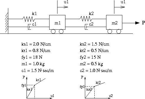
In this example we use Aladdin's matrix language to calculate the load-displacement response of a nonlinear mass-spring system subject to a well-defined external loading. Our analysis will be divided into two parts:
By using the matrix language for the complete analysis, we are really creating a high-level software prototype suitable for testing algorithms and new ideas. This particular example assumes bi-linear hysteretic behavior of the springs. (A reasonable variation on this problem would be to examine the behavior of a system having a Romberg-Osgood stress-strain curve.)
Once everything works, the follow-up implementation would involve a finite element implementation of the modeling mesh and element-level behavior. The second implementation will have improved performance because sections of interpreted code in the first version will now be executed as low-level compiled code in the finite element version.
Section and Material Properties
The lower-half of Figure 1 defines the mass-spring system properties.
Springs 1 and 2 both have a bi-linear force-displacement relationships which follow the kinematic hardening rule . The basic shape of the force-displacement constituitive relationship is defined by the Aladdin variables:
   /* Define bi-linear spring behavior */

   ks1 = 2.0 N/cm;   ks2 = 1.5 N/cm;
   kt1 = 0.8 N/cm;   kt2 = 0.5 N/cm;
   fy1 =  18 N;      fy2 =  15 N;

   Ks = [ks1; ks2];
   Kt = [kt1; kt2];
   Fy = [fy1; fy2];
The undeformed springs start out with an initial stiffness "ks" that lasts until the load exceeds the yield force "fy". The tangent stiffness then changes to "kt". When the loading is reversed, the tangent stiffness switches back to the initial stiffness "ks" until the yielding reappears. The elastic force-displacement range is 2.fy.
External Loads
At each step of the analysis the end-load is incremented by either 1 N or -1 N, depending on whether the load is increasing or decreasing.
The relevant section of Aladdin code is:
   for ( k = 1; k <= total_step ; k = k+1 ) {

      /* define force increment for each step */

      if( k<=20 )           { d_P =  [0 N; 1 N]; }
      if( k>20  && k<=60  ) { d_P = -[0 N; 1 N]; }
      if( k>60  && k<=105 ) { d_P =  [0 N; 1 N]; }
      if( k>105 && k<=155 ) { d_P = -[0 N; 1 N]; }
      if( k>155 && k<=190 ) { d_P =  [0 N; 1 N]; }
      if( k>190 && k<=200 ) { d_P = -[0 N; 1 N]; }
      if( k>200 )           { d_P =  [0 N; 0 N]; }

      P = P + d_P;

      .... details of analysis removed .....
   }
Here d_P is the load increment and P is the external load. The resulting graph of external load versus step number is shown in Figure 2.
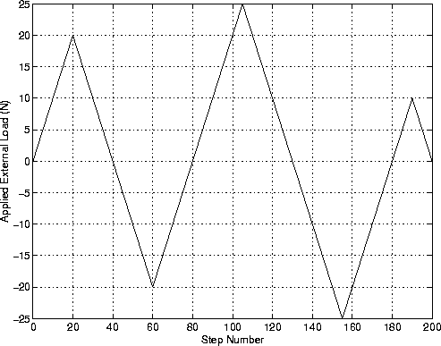
Figure 3 shows the load-deflection curve for springs 1 and 2. Similar force-displacement curves can be drawn for the individual springs of course.
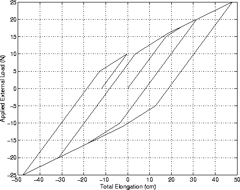
During the first 20 steps of the analysis the external load is incrementally increased from 0 N to 20 N. The system response will be elastic for the first 15 steps -- that is until the external load equals 15 N. The effective stiffness of the mass-spring system prior to first yield is:
    Effective stiffness =  1 / ( 1/ks1 + 1/ks2 )
                        =  6/7 N/cm.
Hence we expect that when the external force equals 15 N, the system displacement will be:
    Displacement at first yield = 15 N / 6/7 N/cm
                                = 17.5 cm.
For external loading between 15 and 18 N, the effective stiffness will be:
    Intermediate effective stiffness =  1/ ( 1/ks1 + 1/kt2 )
                                     =  2/5 N/cm.
Both springs will yield when the external load reaches 18 N. The effective stiffness drops to 4/13 N/cm for externalloads between 18 and 20 N.
From this point on the load-deflection is as shown in Figure 3, but defined by the loading history shown in Figure 2. When the analysis ceases at Step 200, the system will have a -12 cm residual displacement.
Figure 4 shows the notation that we will use for the nonlinear spring state determination.
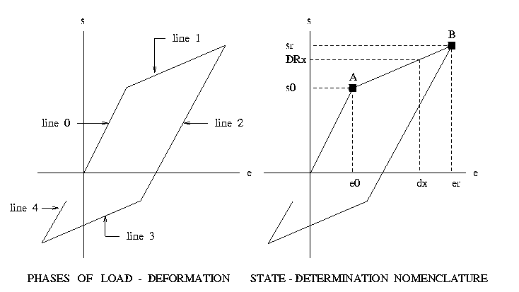
We will use the variables "s" and "e" for the force and displacement at the integration section.
| Variable(s) | |
| DRx dx | Current force and displacement |
| s0 e0 | Force and displacement at the point where the two tangent stiffness lines meet, like point A in Figure 3. |
| sr er | Force and displacement at the point where the last displacement reversal with force, like point B in Figure 3. |
| sx ex | Temporary force and displacement variables used in evaluation of section forces. |
| sx_saved ex_saved sr_saved er_saved | Working arrays that store response from previous analysis step. |
For the bi-linear force-displacement curve:
DRx = sx + kx*( dx - ex )
The state determination can be viewed as a sequence of transitions from lines 0 through 4.
if( yielding[ele][1] == 0 ) then {

    if( abs(dx) <= ey[ele][1] ) then {  /* line 0 on Figure 3         */
        kx = Ks[ele][1];
        sx = 0 N;
        ex = 0 cm;
        yielding[ele][1]  = 0;
        pre_range[ele][1] = 0;
    } else {                            /* move from line 0 to line 1 */
        kx = Kt[ele][1];
        s0[ele][1] = Fy[ele][1]*loading[ele][1];
        e0[ele][1] = ey[ele][1]*loading[ele][1];
        sx = s0[ele][1];
        ex = e0[ele][1];
        yielding[ele][1]  = 1;
        pre_range[ele][1] = 1;
    }

} else {

    .... source code for plastic residual .....

}
The two cases to consider are: (1) the response remains on line 0, and (2) the response moves from line 0 to either of lines 1 or 3.
The array loading[ele][1] is given by:
     if( d_dx >  0 cm ) { loading[ele][1] =  1; }
     if( d_dx <  0 cm ) { loading[ele][1] = -1; }
     if( d_dx == 0 cm ) { loading[ele][1] = pre_load[ele][1]; }
thereby allowing for yielding in both tension and compression.
if( yielding[ele][1] == 0 ) then {

    .... source code for elastic response .....

} else {

    if( pre_load[ele][1] != loading[ele][1] ) then {

        if( pre_range[ele][1] == 1 ) then {
            sr[ele][1] = sx_saved[ele][1];
            er[ele][1] = ex_saved[ele][1];
            kx = Ks[ele][1];
            sx = sr[ele][1];
            ex = er[ele][1];
            pre_range[ele][1] = 0;
        } else {   /* pre_range[ele][1] = 0 */
            if( loading[ele][1]*dx <= loading[ele][1]*er[ele][1] ) then {
                kx = Ks[ele][1];
                sx = sr[ele][1];
                ex = er[ele][1];
                pre_range[ele][1] = 0;
            } else {
                if( loading[ele][1]*ex_saved[ele][1] >= loading[ele][1]*er[ele][1] ) then {
                    kx = Ks[ele][1];
                    sx = sr[ele][1];
                    ex = er[ele][1];
                    pre_range[ele][1] = 0;
                } else {
                    kx = Kt[ele][1];
                    sx = sr[ele][1];
                    ex = er[ele][1];
                    pre_range[ele][1] = 1;
                }
            }
            }

    } else {   /* pre_load[ele][1] == loading[ele][1] */

        if( pre_range[ele][1] == 1 ) then {
            kx = Kt[ele][1];
            sx = s0[ele][1];
            ex = e0[ele][1];
            pre_range[ele][1] = 1;
        } else {  /* pre_range[ele][1] = 0 */

            if( loading[ele][1]*ex_saved[ele][1] <= loading[ele][1]*er[ele][1] ) then {
                if( loading[ele][1]*dx <= loading[ele][1]*er[ele][1] ) then {
                    kx = Ks[ele][1];
                    sx = sr[ele][1];
                    ex = er[ele][1];
                    pre_range[ele][1] = 0;
                } else { /* line 2 -> line 1 */
                    kx = Kt[ele][1];
                    sx = sr[ele][1];
                    ex = er[ele][1];
                    pre_range[ele][1] = 1;
                }
            } else { /* line 4 */
                if( abs(dx-er[ele][1]) <= 2*ey[ele][1] ) then {
                    kx = Ks[ele][1];
                    sx = sr[ele][1];
                    ex = er[ele][1];
                    pre_range[ele][1] = 0;
                } else { /* line 4 -> line 1 */
                    s0[ele][1] = sr[ele][1] + loading[ele][1]*2*Fy[ele][1];
                    e0[ele][1] = er[ele][1] + loading[ele][1]*2*ey[ele][1];
                    kx = Kt[ele][1];
                    sx = s0[ele][1];
                    ex = e0[ele][1];
                    pre_range[ele][1] = 1;
                }
            } /* end of line 4 */
        }
    }
}
Points to note:
pre_load[][]
stores the values of array loading from the previous analysis step.
pre_range [][]
indicates the elastic or plastic status of the previous step. The array element is set to 0 when the previous step in the stress-strain relationship is in elastic range. Conversely, its value is set to 1 if it was in the plastic range.
So why do we need array pre_range[][]?
If the previous step results in plastic range, and in the current step we have a reversal loading case, you know that the tangent stiffness for current step is elastic stiffness. But if it's elastic in previous step, even you have a reversal loading, you can't guarantee that it's elastic or plastic stiffness for this step, because it depends on the size of the displacement increment.
The heart of the force-displacement calculation is contained in the block of code:
/* Define bi-linear spring behavior */

   .... details shown above .....

/* Compute and store displacements for incipient yielding of springs */

   ey = Matrix([2,1]);
   for( ele=1; ele<=2; ele=ele+1 ) {
      ey[ele][1] = Fy[ele][1]/Ks[ele][1];
   }

/* Initial condition, unstressed */

   P   = [0 N;   0 N];       /* structure force           */
   p   = [0 cm; 0 cm];       /* structure displacement    */
   PR  = [0 N;   0 N];       /* structure resisting force */
   PRe = [0 N;   0 N];       /* element resisting force   */

   Q_saved  = [0  N; 0  N];  /* matrix of element forces        */
   q_saved  = [0 cm; 0 cm];  /* matrix of element displacements */

/* initialize flags, stresses and strains before applying any load step */

   index = [0;0];  /* index for loading flag   */
   flag1 = [0;0];  /* yielding at load step k  */
   flag2 = [0;0];  /* pre_range at load step k */
   flag3 = [0;0];  /* pre_load at load step k  */

   yielding  = [0;0];
   pre_range = [0;0];
   pre_load  = [0;0];
   loading   = [0;0];
   sr = [0 N;   0 N];
   er = [0 cm; 0 cm];
   s0 = [0 N;   0 N];
   e0 = [0 cm; 0 cm];

   sr_saved = [0 N;   0 N];
   er_saved = [0 cm; 0 cm];
   s0_saved = [0 N;   0 N];
   e0_saved = [0 cm; 0 cm];
   sx_saved = [0 N;   0 N];
   ex_saved = [0 cm; 0 cm];

/* transformation matrix Lele, d_q = Lele*d_p[ele] for each element    */
/* transform structural displacements d_p to element deformations d_q  */

   Rigid = [-1,1];
   Transform = [1,0;0,1];
   L = Rigid*Transform;

/* temporary matrix to store element tangent stiffness Ks at each step */

   tangent = [Ks[1][1] ; Ks[2][1]];

/* force interpolation matrices b(x), D(x) = b(x)*Q */
/* relate section force D(x) with element force Q */

   bx = 1;

/* assemble initial structure tangent stiffness matrix BigK */

   BigK = [ Ks[1][1]+Ks[2][1], -Ks[2][1];
                    -Ks[2][1],  Ks[2][1] ];

/* Increase external load, structure determination */

tol = 0.00001; total_step = 400;
for ( k=1; k<=total_step ; k=k+1 ) {

   /* Define incremental loading */

      .... details shown above ....

   err = tol+1;
   while( err > tol )  { /* i-th Newton-Raphson iteration */

      /* compute displacement increment */

      d_p = Solve( BigK, d_P);
      p   = p + d_p;

      /* Element level state determination */

      for( ele = 1; ele <= 2; ele = ele + 1 ) {

         /* Retrieve element level displacements   */

         if( ele==1 ) {
             d_pe = [       0 m; d_p[1][1] ];
         }
         if( ele==2 ) {
             d_pe = [ d_p[1][1]; d_p[2][1] ];
         }

         /* Retrieve values from previous iteration */

         Q  = Q_saved[ele][1];      /* element-level forces           */
         q  = q_saved[ele][1];      /* element-level displacements    */
         Dx = bx*Q;                 /* section forces                 */
         dx = bx*q;                 /* section displacements          */
         K  = tangent[ele][1];      /* tangent stiffness of element   */
         kx = tangent[ele][1];      /* tangent stiffness of element   */
         fx = 1/kx;                 /* tangent flexibility of element */

         rx  = 0 cm;
         DUx = 1E+7 N;

         /* Increment element deformation */

         d_q = QuanCast(L*d_pe);
         q   = q + d_q;

         /* iterative loop for convergence of element forces */

         while( abs(DUx) > 0.00001 N ) {

            d_Q = K*d_q;          /* element force increment */
            Q   = Q + d_Q;        /* update element force    */

            /* determine the section force increments           */
            /* repeat for all integration points of the element */

            d_Dx = bx*d_Q;        /* section force increment           */
            d_dx = rx + fx*d_Dx;  /* section deformation increment     */
            Dx = Dx + d_Dx;       /* update section force              */
            dx = dx + d_dx;       /* update section deformation vector */

            /* Section level state determination */

               ... compute "kx", "sx", and "ex" ....

            /* Calculate stress and flexibility  */

            fx  = 1/kx;             /*                              */
            DRx = sx + kx*(dx-ex);  /*                              */

            DUx = Dx - DRx;         /* section unbalanced force     */
            rx  = fx*DUx;           /* section residual deformation */

            /* finish for all integration points of the element      */
            /* update the element flexibility and stiffness matrices */

            F = bx*fx*bx;
            K = 1/F;

            /* check for element convergence */

            s = bx*rx;   /* element residual deformation */
            d_q = -s;
         }

         /* Save element level forces and displacements */

         Q_saved[ele][1] = Q;
         q_saved[ele][1] = q;

         tangent[ele][1] = K; /* element stiffness Ke =LT*K*L=[K,-K;-K,K]    */
         PRe[ele][1] = Q;     /* element resistant force PRe = LT*Q = [-Q;Q] */
      }

      /* assemble structure resistant force */

      PR[1][1] = PRe[1][1] - PRe[2][1];
      PR[2][1] = PRe[2][1];

      /* assemble new structure stiffness */

      BigK[1][1] =  tangent[1][1] + tangent[2][1];
      BigK[1][2] = -tangent[2][1];
      BigK[2][1] = -tangent[2][1];
      BigK[2][2] =  tangent[2][1];

      d_P = P - PR;
      err = L2Norm(d_P);

   }  /* i-th iteration in Newton-Raphson while loop */
}
Figure 5 shows the elastic and inelastic strain energy in a typical nonlinear system.
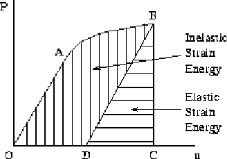
During loading, the work done is equal to the area under the curve (i.e., area OABCDO). When the load is removed the load-deflection diagram follows line BD. A permanent elongation OD remains when point B is beyond the elastic limit. Thus, the elastic strain energy recovered during unloading is represented by the shaded triangle BCD. Area OABDO represents energy that is lost in the process of permanently deforming the bar. This energy is known as the inelastic (or plastic) strain energy.
Summary of Results
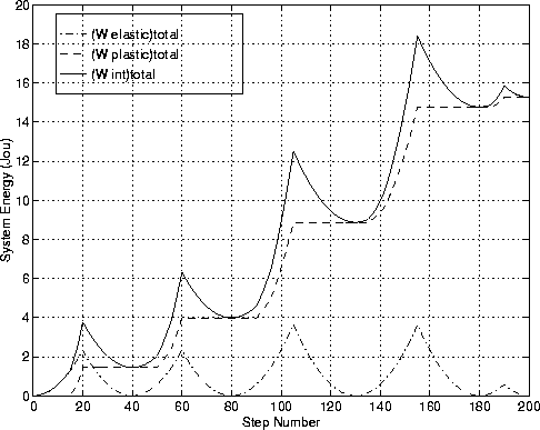
Figure 6 shows components of strain-enegy for springs 1 and 2. Similar force-displacement curves can be drawn for the individual springs.
Solution Procedure
In the static analysis, a Newton-Raphson procedure is used to calculate the load-deflection response of this spring system. We also calculate the elastic and plastic components of energy of the spring elements. Except for the spring properties and strain energy calculation, the input file is almost the same as for the composite bar example presented in the preceding chapter.
The abbreviated input file is:
/* allocate the matrices for storing energy calculations */

   system_energy  = ColumnUnits( Matrix([total_step+1,4]), [Jou] );
   element_energy = ColumnUnits( Matrix([total_step+1,4]), [Jou] );

/* Increase External Load */

   for ( k = 1; k <= total_step ; k = k+1 ) {

   /* define force increment for each step */

      .... details of load increment found above ....

      element_energy[k+1][1] = element_energy[k][1];
      element_energy[k+1][3] = element_energy[k][3];

   /* i-th Newton-Raphson Iteration */

      index[1][1] = 1;   index[2][1] = 1;
      err = tol+1;
      while( err > tol ) {

         d_p = Solve(BigK,d_P);
         p = p + d_p;

         /* state determination for each element */

         for( ele=1;ele<=2;ele=ele+1 ) {

         ...... details about retrieving data from (j-1) ......

         q = q + d_q;

         /* element converge, j */

            while( abs(DUx) > 0.00001 N ) {

              ...... details of checking element convergence  ...... }
              ...... details of updating data at loop j ......

             /* energy calculations for each element ele */

            element_energy[k+1][2*ele-1] = element_energy[k+1][2*ele-1]
                           + 0.5*(Q_saved[ele][1]+Q)*(q-q_saved[ele][1]);
            element_energy[k+1][2*ele]   = 0.5*Q*Q/Ks[ele][1];
         }

      /* assemble structure resistant force */

         ...... details of assembling structure resistant force ......

      /* assemble new structure stiffness */

         ...... details of assembling new structure stiffness ......

      d_P = P - PR;
      err = L2Norm(d_P);

   }  /* i-th iteration in Newton-Raphson while loop */

      ...... details of storing response removed ......

      ...... details of updating element history ......

   /* Reassemble the System Energy */

      system_energy[k+1][1] = system_energy[k][1] +
                              0.5*(result[k+1][1]+result[k][1])*(result[k+1][2]-result[k][2]);
      system_energy[k+1][2] = element_energy[k+1][1]+element_energy[k+1][3];
      system_energy[k+1][3] = element_energy[k+1][2]+element_energy[k+1][4];
      system_energy[k+1][4] = system_energy[k+1][2] - system_energy[k+1][3];
   }
Points to note:
We now repeat the system analysis assuming that the load is incremented in time steps of only 0.01 seconds. The total loading time is 2 seconds. The system response is computed for a total of 4 seconds using the Newmark Integration algorithm with average acceleration across the time steps.
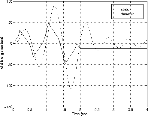
Figure 7 is a comparison of the static and dynamic displacement responses versus step no/time.
First Mode of Vibration
Figure 8 shows the change in the first-mode period versus time during the dynamic analysis.
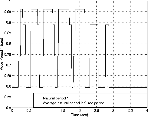
The time-variation in the first and second modes of vibration is computed by simply inserting:
   eigen = Eigen(BigK, BigM, [2]);
   eigenvalue  = Eigenvalue(eigen);

   result[1][7] = 2*PI/sqrt( eigenvalue[1][1] );
   result[1][8] = 2*PI/sqrt( eigenvalue[2][1] );
into the main loop of the time-history calculation. The 7th and 8th columns of "response" store the first and second mode periods versus step no.
System Energy
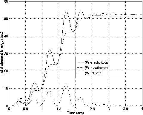
We also calculate the strain energy, elastic and plastic energies of the spring elements, and the natural periods of the system throughout the dynamic analysis. See Figure 9.
Static Analysis
Dynamic Analysis