 Cantilever Beam with Material Nonlinearity
 Cantilever Beam with Material Nonlinearity
[ Problem Statement ]
[ Finite Element Mesh ]
[ Displacements ]
[ Rotations ]
[ Curvature ]
[ Input/Output Files ]
You will need Aladdin 2.0 to run this problem.
Figure 1 shows a two dimensional cantilever beam that carries a monotonically increasing point load at its free end.
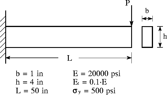
The cantilever is constructed from a material having bi-linear behavior. The section dimensions and material properties are as shown in the lower half of Figure 1. In this example we will compute:
Nodes and Elements
The block of code:
   /* Generate grid of nodes for f.e. model */

   x = 0 in; y = 0 in;
   for( node=1 ; x<=50in ; node=node+1 ) {
      AddNode( node, [x, y] );
      x = x + 5 in;
   }

   /* Attach elements to grid of nodes */

   for( elmt_no = 1 ; elmt_no <= total_elmt ; elmt_no = elmt_no + 1) {
      AddElmt( elmt_no, [ elmt_no, elmt_no+1 ], "name_of_elmt_attr" );
   }
generates the line of beam finite elements shown in the upper half of Figure 2.
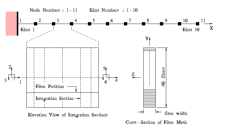
The cantilever is modeled with 10 "FIBER_2D" elements, each element contains 40 fibers that stretch along the length of the finite element. Behavior of the element along its length is computed via integration at 5 sections. The overall deformations in each element are described by only six degrees of freedom, however. After the wall support has been fully-fixed, i.e.,
FixNode( 1, [ 1, 1, 1] );
the structural model has 30 d.o.f.
Finite Element Attributes
The finite element attribute declaration:
   ElementAttr("name_of_elmt_attr") { type     = "FIBER_2D";
                                      section  = "mysection";
                                      material = "mymaterial";
                                      fiber    = "fibername";
                                    }
establishes the finite element type, FIBER_2D, and the section, material, and fiber layout for the finite element.
Section and Material Properties
The section and material properties are given by:
   h = 4.0 in;  b = 1.0 in;
   ks = 20000 psi;  kt = 0.1*ks;  fy = 500 psi;

   SectionAttr("mysection") { area  = b*h;
                              width = b;
                              depth = h;
                              shear_factor  = 1.2;
                            }

   MaterialAttr("mymaterial") { density = 2 lbf*sec^2/in/in^3;
                                poisson = 0.25;
                                E     = ks;
                                Et    = kt;
                                yield = fy;
                                shear_yield = 10000*fy;
                              }
Fiber Geometry
The nonlinear beam behavior is modeled with a stack of 40 fiber elements, as shown in the cross section view of the FIBER_2D finite element. This fiber layout is generated with:
   no_fiber = 40; no_fiber_type = 1; dh = h/no_fiber;

   fcoord = Matrix([ 1, no_fiber ]);
   farea  = Matrix([ 1, no_fiber ]);
   fmap   = Matrix([ 1, no_fiber ]);

   for( i=1 ; i <= no_fiber ; i=i+1 ) {
      fcoord[1][i] = h/2 - dh/2 - (i-1)*dh;
      farea[1][i]  = b*h/no_fiber;
      fmap[1][i]   = 1;
   }

   fattr  = Matrix([ 3, no_fiber_type ]);
   for( j=1 ; j <= no_fiber_type ; j=j+1 ) {
        fattr[1][j] = ks;
        fattr[2][j] = kt;
        fattr[3][j] = fy;
   }

   FiberAttr(no_fiber, "fibername" ){ FiberMaterialAttr = fattr;
                                      FiberCoordinate   = fcoord;
                                      FiberArea         = farea;
                                      FiberMaterialMap  = fmap;
                                    }
In this particular example, "fcoord [i][1]" stores the y-coordinate of the i-th fiber element. All of the fibers have a cross section area:
b*h/no_fiber = 1 in * 4 in / 40 fibers = 0.1 in^2.
and the same values of "ks", "fy" and "kt".
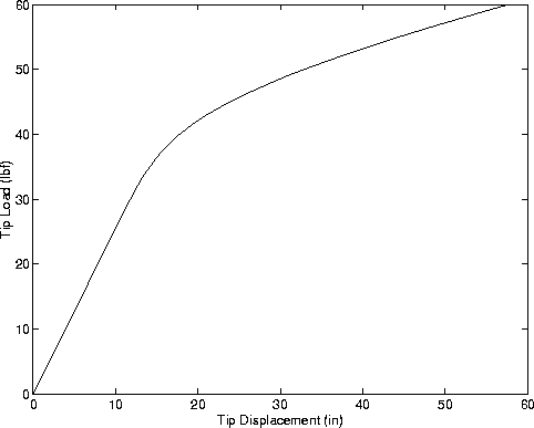
Figure 3 shows the vertical displacement of the cantilever tip (in) versus applied load (lbf).
Displacement Analysis
The abbreviated block of code:
   total_step = 60;
   for( step=1 ; step <= total_step ; step=step+1 ) {

      dPk = [ 0 lbf, 1 lbf, 0 lbf*in ];
      NodeLoad( total_node, dPk );

      P_new = ExternalLoad();
      dP    = P_new - P_old;
      P_old = P_new;

      /* Newton-Raphson Iteration for State Determination */

      while( L2Norm(dP) > 0.001 ) {

         dp    = Solve( Ks, dP );
         displ = displ + dp;

         ElmtStateDet( dp );

         Ks = Stiff();               /* Compute new stiffness    */
         PR = InternalLoad( displ ); /* Compute internal load    */
         dP = P_new - PR;            /* Compute unbalanced force */

      }

      /* Update element history data */

      UpdateResponse();

      /* Save external load, and tip displacement and rotation */

      tip_response[step+1][1] = P_new[max_dof][1];
      tip_response[step+1][2] = displ[max_dof][1];
      tip_response[step+1][3] = displ[max_dof+1][1];

      /* store all element results every 10 steps */

      ..... details removed .....

   }
systematically increases the applied load at the cantilever tip from 1 lbf to 60 lbf in increments of 1 lbf, and computes and saves the beam response due the external loads.
The built-in function "ElmtStateDet()" to performs of the element state determinations. Similarly, after each load step finished, the element stress, strain, and material information is updated by the built-in function "UpdateResponse()".
The matrix "tip_response" stores the applied external load, tip displacement, and tip rotation for each step, including the initial non-loaded status. Matices "displacement" and "rotation" store the nodal displacement and rotation once every 10 steps.
Incipient Yielding
We can use elementary structural mechanics theory to estimate the external load that will cause incipient yielding of the beam fiber.
Assuming that the distribution of stresses in the beam can be approximated with:
            M . y
    sigma = -----  and  M = P.L  and  I = 1/12 b.h^3.
              I
then first yielding of the fibers occurs in the outer layers of the beam at the fixed end when the tip load reaches 26.7 lbf. The coordinates of first yield are x = 0 in and y = 2 in and y = -2 in.
Of course the beam deflection grows rapidly after yielding.
Accuracy of Deflection Calculations
This fiber element includes effects of shear deformation. When P = 20 lbf, for example, the calculated tip deflection is 7.85489 in. Theoretical considerations [1] indicate that the exact solution for the vertical displacement of the cantilever is:
         P.L^3                       f_s.P.L
   v_b = ----- = 7.8125 in     v_s = ------- = 0.0375 in.
         3.EI                        G.A.
The combined deflection is:
v_t = v_b + v_s = 7.85 in.
where "f_s" is the shear factor. Neglecting the shear deformation effects results in a relative deflection error of: If the relative shear deformation effects are not considered, like in the FRAME_2D element, the relative numerical error will be
          v_s
    err = ---  = 0.478 %
          v_t
The relative numerical error for this example is
          delta - v_t
    err = ----------- = 0.0623 %
              v_t
which is much less than the traditional plane frame element. In this example the numerical error of FRAME_2D is small because the beam is slender (i.e., h/L < 1/10). Shear deformation would make a much larger contribution to the overall displacement for deep beams with large h/L ratios.
Contours of Beam Displacement
Figure 4 shows how the deflected shape of the beam changes as a function of applied load.
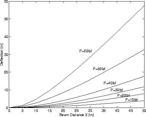
We only display the cantilever shape for applied loads 0 lbf, 10 lbf, 20 lbf and so forth. The block of Aladdin code:
    flag = flag+1;
    if( flag == 0 ) {

        for( node=2 ; node<=total_node ; node=node+1 ) {
             node_displacement         = GetDispl( [node] , displ);
             displacement[node][index] = node_displacement[1][2];
             rotation[node][index]     = node_displacement[1][3];
        }

        for(elmt_no=1 ; elmt_no<=total_elmt ; elmt_no=elmt_no+1){
            curvature[elmt_no][index] = (rotation[elmt_no+1][index]
                                       - rotation[elmt_no][index])/(5 in);
        }
        flag  = -10;
        index = index+1;
     }
uses the "flag" variable to detect increments of 10 lbf external loading. The vertical displacement and rotation of nodes 2 through 10 are retrieved and saved in the arrays "displacement" and "rotation", respectively.
Figure 5 shows the tip rotation as a function of applied tip load.
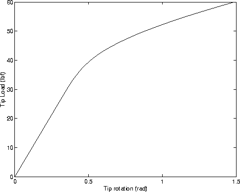
You should observe that this curve is smooth even though the material behavior is bi-linear. This behavior can be attributed to the gradual spread of fiber yielding and from the exterior fibers towards the beam centroid.
We can easily calculate the curvature for fiber element "i" by
                theta_i+1 - theta_i
     kappa_i =  -------------------
                       L_i
because curvature along an element is constant. Here "L_i" is the length of element "i", "theta_i" and "theta_i+1" are the end rotations. The results are shown in Figure 6.
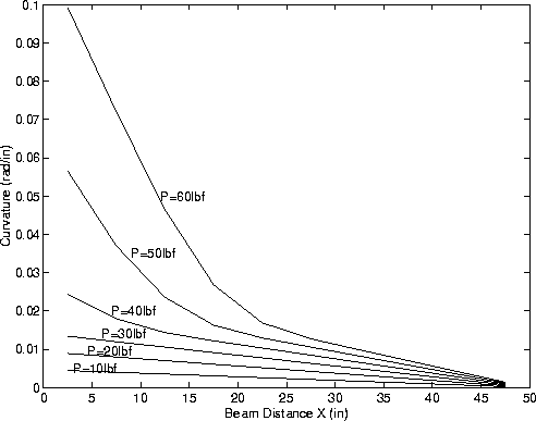
You should observe that in regions of elastic behavior - this includes all of the contours for loading 10 lbf and 20 lbf -- the element curvature will be linearly proportional to the section bending moment. The element curvature will increase significantly when the extreme element fiber yields -- one can therefore estimate which elements are subject to partial and almost total section plasticity.
References