[ Problem Statement ]
[ Finite Element Mesh ]
[ Eigenvalue Analysis ]
[ Dynamic Analysis ]
[ Displacements ]
[ Ductility Demand ]
[ Energy Balance Calculations ]
[ Input/Output Files ]
You will need Aladdin 2.0 to run this problem.
Four-Span Isolated Bridge
This example uses ALADDIN for a three dimensional nonlinear time-history analysis of a 4 span base isolated highway bridge. The bridge model is taken from the text of Priestley et al. [1].
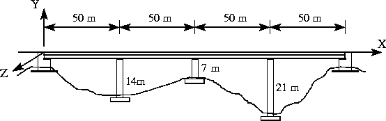
Figure 1 is a longitudinal view of the bridge geometry, having 2 abutment supports and three columns of irregular height. The abutments are assumed to have infinite strength.
In this example we:
Section and Material Properties
The pier and deck section properties are shown in Figure 2.
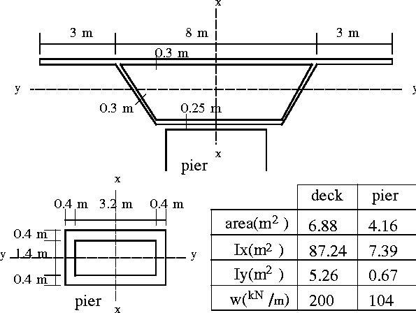
All of the piers have identical cross sectional properties, but the reinforcement is detailed so that the piers have approximately the same lateral force resistance.
Capacities of the piers and isolators are listed in Table 1.
| Secant Stiffness (kN/m) | Yield Strength (kN) | |
| Isolators 1 and 5 | 5300 | 2100 |
| Isolator 2 | 16100 | 2100 |
| Isolator 3 | 11500 | 2100 |
| Isolator 4 | 47000 | 2100 |
| Pier 2 | 30700 | |
| Pier 3 | 124400 | |
| Pier 4 | 13650 |
The isolators are assumed to have elastic-perfectly plastic behavior, which means no strain hardening after yielding.
How does Base Isolation of Highway Bridges work?
When a seismic base isolator is installed between the top of a bridge column and beneath the deck structure, the parameters of the column combine with those of the isolator. The overall characteristics of the superstructure and isolation system reflect a combination of individual composite dynamic parameters.
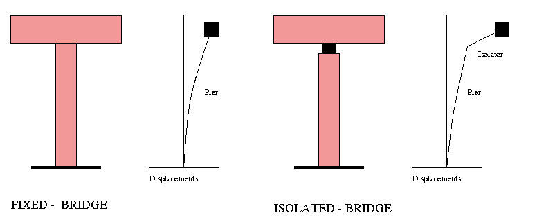
For most practical situations, the superstructure mass is much greater than the column mass, and hence the first mode of vibration is dominated by displacements of the superstructure. The second mode, in comparison, involves lateral motion of the top of the column with little movement of the superstructure (see, for example, Figure 4).
The finite element mesh is shown in Figure 5.
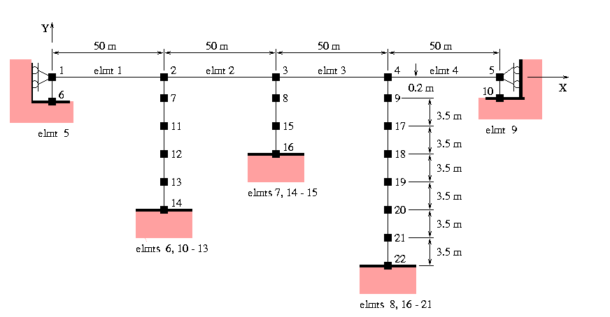
The finite element mesh has 22 nodes and 21 elements. The latter are a combination of FRAME_3D and FIBER_3D elements, as detailed in Table 2.
| Element Nos | Description | Element Type |
| 1 to 4 | Bridge Deck Attribute | FRAME_3D |
| 5 and 9 | Isolator Attribute 1 | FIBER_3D |
| 6 | Isolator Attribute 2 | FIBER_3D |
| 7 | Isolator Attribute 3 | FIBER_3D |
| 8 | Isolator Attribute 4 | FIBER_3D |
| 10 to 13 | Column 2 | FRAME_3D |
| 14 and 15 | Column 3 | FRAME_3D |
| 16 to 21 | Column 4 | FRAME_3D |
The deck and columns are modeled with elastic 3-D frame elements (i.e., element type FRAME_3D). Only the isolators are modeled as 3-D nonlinear fiber elements with bi-linear shear-displacement response (i.e., element type FIBER_3D).
The lower ends of the piers and abutments are fully fixed. We also assume that there are no longitudinal deformations and twisting at the both ends of the bridge deck. In total there are 21 elements, 8 different element attributes and 98 degrees of freedom in this model.
Nodes and Elements
The block of code:
H2    = 14 m;
H3    =  7 m;
H4    = 21 m;
iso_h = 20 cm;

/* Assemble mesh of nodes and elements */

   total_node = 0;
   x = 0 m;  y = 0 m;  z = 0 m;
   for( node_no=total_node+1 ; x<=200m ; node_no=node_no+1 ) {
       AddNode( node_no, [x,y,z] );
       x = x + 50 m;
   }

   total_node = node_no-1;
   x = 0 m;  y = -iso_h;  z = 0 m;
   for( node_no=total_node+1 ; x<=200m ; node_no=node_no+1 ) {
       AddNode( node_no, [x,y,z] );
       x = x + 50 m;
   }

   total_node = node_no-1;
   x = 50 m;  y = -iso_h-3.5m;  z = 0 m;
   for( node_no=total_node+1 ; y>=-(iso_h+H2) ; node_no=node_no+1 ) {
       AddNode( node_no, [x,y,z] );
       y = y - 3.5 m;
   }

   total_node = node_no-1;
   fix2       = total_node;
   x = 100 m;  y = -iso_h-3.5m;  z = 0 m;
   for( node_no=total_node+1 ; y>=-(iso_h+H3) ; node_no=node_no+1 ) {
       AddNode( node_no, [x,y,z] );
       y = y - 3.5 m;
   }

   total_node = node_no-1;
   fix3       = total_node;
   x = 150 m;  y = -iso_h-3.5m;  z = 0 m;
   for( node_no=total_node+1 ; y>=-(iso_h+H4) ; node_no=node_no+1 ) {
       AddNode( node_no, [x,y,z] );
       y = y - 3.5 m;
   }
defined the (x,y,z) coordinate position for the 22 nodes in the finite element model. Elements are attached to the nodes in three stages -- the block of code:
   total_node = node_no-1;
   fix4       = total_node;

   total_elmt = 0;
   for( elmt_no=total_elmt+1 ; elmt_no<=4 ; elmt_no=elmt_no+1 ) {
       AddElmt( elmt_no, [elmt_no, elmt_no+1], "deck_attr" );
   }
attaches the elements for the bridge deck. The base isolator finite elements are added to the mesh with:
   AddElmt(  5, [1,6],  "isolator_attr1" );
   AddElmt(  6, [2,7],  "isolator_attr2" );
   AddElmt(  7, [3,8],  "isolator_attr3" );
   AddElmt(  8, [4,9],  "isolator_attr4" );
   AddElmt(  9, [5,10], "isolator_attr1" );
Finally the finite elements for the three columns are added to the mesh with:
   total_elmt = 9;
   node_no = fix2 - H2/(3.5m) + 1;
   AddElmt( total_elmt+1, [7, node_no], "column_attr2" );

   total_elmt = total_elmt+1;
   for( elmt_no = total_elmt+1 ; node_no < fix2 ; elmt_no=elmt_no+1 ) {
       AddElmt( elmt_no, [node_no, node_no+1], "column_attr2" );
       node_no = node_no+1;
   }

   total_elmt = elmt_no-1;
   bot_elmt2  = total_elmt;
   node_no    = fix3 - H3/(3.5m) + 1;
   AddElmt( total_elmt+1, [8, node_no], "column_attr3" );
   total_elmt = total_elmt+1;
   for( elmt_no=total_elmt+1 ; node_no < fix3 ; elmt_no=elmt_no+1 ) {
       AddElmt( elmt_no, [node_no, node_no+1], "column_attr3" );
       node_no = node_no+1;
   }

   total_elmt = elmt_no-1;
   bot_elmt3  = total_elmt;
   node_no    = fix4 - H4/(3.5m) + 1;
   AddElmt( total_elmt+1, [9, node_no], "column_attr4" );
   total_elmt = total_elmt+1;
   for( elmt_no=total_elmt+1 ; node_no < fix4 ; elmt_no=elmt_no+1 ) {
       AddElmt( elmt_no, [node_no, node_no+1], "column_attr4" );
       node_no = node_no+1;
   }

   total_elmt = elmt_no-1;
   bot_elmt4  = total_elmt;
with blocks of Aladdin code that walk along the bridge deck, then the isolator level, and finally down each of the nodal lines for the bridge supports.
Material and Section Properties
The following block of code:
   ElementAttr("deck_attr") { type     = "FRAME_3D";
                              section  = "deck_sec";
                              material = "deck_mat";
                            }
   SectionAttr("deck_sec")  { Iyy = 103.77 m^4; Izz = 5.26 m^4;
                              J       = 16.13 m^4;
                              area    = 6.88 m^2;
                              unit_weight = 200 kN/m;
                            }
   MaterialAttr("deck_mat") { poisson = 0.25;
                              E       = 2.3e7 kN/m^2;
                            }

   b  = 2.2    m;  h = 4.0    m;
   Ix = 7.39 m^4; Iy = 0.67 m^4;
   K2 =       30700 kN/m; K3 =      124400 kN/m; K4 = 13650 kN/m;
   E2 = K2*H2*H2*H2/3/Ix; E3 = K3*H3*H3*H3/3/Ix; E4 = K4*H4*H4*H4/3/Ix;

   ElementAttr("column_attr2") { type     = "FRAME_3D";
                                 section  = "col_sec";
                                 material = "col_mat2";
                               }

   ElementAttr("column_attr3") { type     = "FRAME_3D";
                                 section  = "col_sec";
                                 material = "col_mat3";
                               }

   ElementAttr("column_attr4") { type     = "FRAME_3D";
                                 section  = "col_sec";
                                 material = "col_mat4";
                               }

   SectionAttr("col_sec") { area  = 4.16 m^2;
                            width = h;  depth = b;
                            Iyy   = Ix; Izz   = Iy;
                            unit_weight  = 104 kN/m;
                            shear_factor = 1.0;
                          }

   MaterialAttr("col_mat2") { poisson = 0.25;  E = E2; }
   MaterialAttr("col_mat3") { poisson = 0.25;  E = E3; }
   MaterialAttr("col_mat4") { poisson = 0.25;  E = E4; }

   h = 50 cm;
   b = 50 cm;
   E_lead = 356200 kN/m^2;
   G1  = 4240 kN/m^2;  G2 = 12880 kN/m^2;   G3 = 9200 kN/m^2;   G4 = 37600 kN/m^2;
   fvy = 8400 kN/m^2;

   ElementAttr("isolator_attr1") { type     = "FIBER_3D";
                                   section  = "iso_sec";
                                   material = "iso_mat1";
                                   fiber    = "iso_fib";
                                 }

   ElementAttr("isolator_attr2") { type     = "FIBER_3D";
                                   section  = "iso_sec";
                                   material = "iso_mat2";
                                   fiber    = "iso_fib";
                                 }

   ElementAttr("isolator_attr3") { type     = "FIBER_3D";
                                   section  = "iso_sec";
                                   material = "iso_mat3";
                                   fiber    = "iso_fib";
                                 }

   ElementAttr("isolator_attr4") { type     = "FIBER_3D";
                                   section  = "iso_sec";
                                   material = "iso_mat4";
                                   fiber    = "iso_fib";
                                 }

   SectionAttr("iso_sec") { area  = b*h;
                            width = b;
                            depth = h;
                            unit_weight  = 0.0001 kN/m;
                            shear_factor = 1.0;
                          }

   MaterialAttr("iso_mat1") { poisson = 0.25; G = G1; Gt = 0.001*G1; shear_yield = fvy/2; }
   MaterialAttr("iso_mat2") { poisson = 0.25; G = G2; Gt = 0.001*G2; shear_yield = fvy; }
   MaterialAttr("iso_mat3") { poisson = 0.25; G = G3; Gt = 0.001*G3; shear_yield = fvy; }
   MaterialAttr("iso_mat4") { poisson = 0.25; G = G4; Gt = 0.001*G4; shear_yield = fvy; }

   no_fiber = 4;
   iso_fcoord = Matrix([ 2, no_fiber ]);
   iso_farea  = Matrix([ 1, no_fiber ]);
   iso_fmap   = Matrix([ 1, no_fiber ]);

   iso_fcoord[1][1] =  b/4;
   iso_fcoord[2][1] =  h/4;
   iso_fcoord[1][2] = -b/4;
   iso_fcoord[2][2] =  h/4;
   iso_fcoord[1][3] =  b/4;
   iso_fcoord[2][3] = -h/4;
   iso_fcoord[1][4] = -b/4;
   iso_fcoord[2][4] = -h/4;

   for( i=1 ; i <= no_fiber ; i=i+1 ) {
      iso_farea[1][i]  = b*h/no_fiber;
      iso_fmap[1][i]   = 1;
   }

   iso_fattr = Matrix([ 3, 1 ]);
   iso_fattr[1][1] = E_lead;
   iso_fattr[2][1] = E_lead;
   iso_fattr[3][1] = fvy*1e6;

   FiberAttr( no_fiber, "iso_fib" ) { FiberMaterialAttr = iso_fattr;
                                      FiberCoordinate   = iso_fcoord;
                                      FiberArea         = iso_farea;
                                      FiberMaterialMap  = iso_fmap;
                                    }
is Aladdin code for the element, section and material properties defined in Table 1 and Figure 2.
Boundary Conditions
The following block of code:
   FixNode(   1, [1,0,0,1,0,0]);
   FixNode(   5, [1,0,0,1,0,0]);
   FixNode(   6, [1,1,1,1,1,1]);
   FixNode(  10, [1,1,1,1,1,1]);
   FixNode(fix2, [1,1,1,1,1,1]);
   FixNode(fix3, [1,1,1,1,1,1]);
   FixNode(fix4, [1,1,1,1,1,1]);
restrains nodes 1 and 5 in the horizontal and rotational directions, applies full-fixity to nodes 6 and 10 at the abutments, and full-fixity to the base of the bridge column supports at nodes 14, 16 and 22.
The following fragment of code shows the essential details of code needed to compute the first two modes of vibration, and their natural periods.
   /* Form stiffness matrix and mass matrix */

   stiff = Stiff();
   mass  = Mass([1]);

   /* Compute first two eigenvalues, periods, and eigenvectors */

   no_eigen    = 2;
   eigen       = Eigen(stiff, mass, [no_eigen]);
   eigenvalue  = Eigenvalue(eigen);
   eigenvector = Eigenvector(eigen);

   T1 = 2*PI/sqrt( eigenvalue[1][1] );
   T2 = 2*PI/sqrt( eigenvalue[2][1] );
The first mode of vibration for both the non-isolated and isolated bridges is shown in the three dimensional plots of Figures 6 and 7,
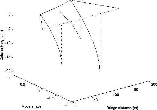
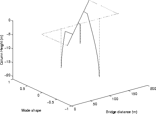
From Figure 6 we see that the non-isolated bridge deck has a "sine curve" first mode deformation. The columns deform elastically. For the isolated bridge, the deck undergoes a rigid body displacement. Most of the deformations in the piers occur at isolators. Also note that the natural periods have been extended significantly from 0.71 sec to 2.02 sec.
Earthquake Ground Motion
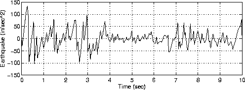
We choose the 1940 El Centro S00E record (see Figure 4) as the input earthquake with the peak ground acceleration scaled to 0.5g.
The deck and piers are assumed to remain elastic during the dynamic responses.
The earthquake ground motion is defined by the block of code:
   Elcentro1 = ColumnUnits( [
     14.56;    13.77;     6.13;     3.73;     1.32;    -6.81;   -16.22;   -22.41;
    -26.67;   -24.10;   -21.86;   -14.02;    -1.62;     1.67;    18.12;    39.26;

     .... details of ground acceleration record removed ....

     -3.05;    -6.01;    -6.08;    -6.40;    -6.70;    -5.70;    -6.14;    -8.41;
    -10.05;   -12.35;   -15.72;     0.00
     ], [cm/sec/sec] );
Each number in the array Elcentro1 corresponds to the digitized ground motion acceleration measured in cm/sec/sec and spaced at 0.02 seconds.
Nonlinear Finite Element Procedure
We now extend the previous analysis to time-history analysis. The time-history analysis assumes equivalent viscous damping of 5% in the form of Rayleigh damping. A second time-history analysis is computed for a non-isolated bridge, thereby enabling comparison of the isolated and non-isolated responses, and assessment of the benefits of base isolation.
The following script of code shows the essential details of the non-linear Newmark analysis:
   while(stepno < total_stepno) {

      /* Update time and step no */

      time   = time + dt;
      stepno = stepno + 1;

      print "*** Start at step  ", stepno, " : TIME = ", time, "\n";

      /* Compute effective incremental loading */

      if( stepno <= dimen[1][1] ) then { P_ext = -mass*r*Elcentro[stepno][1]; }
                                  else { P_ext = -mass*r*(0.0 m/sec/sec); }

      dPeff = P_ext-P_old + ((4/dt)*mass + 2*damp)*velocity + 2*mass*accel;

      /* while loop to check converge, Keff*U = Peff */

      dp  = displ - displ;
      err = 1 + tol;

      ii = 1;
      while( err > tol ) {

         /* Compute effective stiffness from tangent stiffness */

         Keff = stiff + (2/dt)*damp + (4/dt/dt)*mass;

         /* Solve for d_displacement, d_velocity */

         dp_i = Solve( Keff, dPeff);
         dp = dp + dp_i;
         dv = (2/dt)*dp - 2*velocity;

         /* Compute displacement, velocity */

         new_displ    = displ + dp;
         new_velocity = velocity + dv;

         /* Compute incremental displacement and internal load using old stiffness */

         dFs = stiff*dp_i;
         Fs_i = Fs_i + dFs;
         if( ii==1 ) {
            x = L2Norm(dFs);
            if( x==0 ) {x=1;}
         }

         /* Check material yielding and compute new stiffness */

         ElmtStateDet( dp_i );
         stiff = Stiff();

         /* Compute new internal load, damping force, and acceleration */

         Fs = InternalLoad( new_displ );
         Fd = damp*new_velocity;
         new_accel = mass_inv*( P_ext-Fs-Fd );

         /* Calculate the unbalance force, and error percentage */

         P_err = Fs_i - Fs;
         y     = L2Norm(P_err);
         err   = y/x;

         /* Assign new effective incremental load */

         dPeff   = P_err;
         displ_i = new_displ;
         Fs_i    = Fs;

         print "in While Loop" ,ii, ", P_err =" ,y, ", err =" ,err, "\n";
         ii = ii+1;
         if( ii > 23 ) { flag=1; err=tol; }
      }

      /* Calculate the energy balance, Wint(n+1) + T(n+1) = Wext(n+1) */
      /*                                                              */
      /* [1] column 1 is internal work by stiffness                   */
      /* [2] column 2 is internal work by damping                     */
      /* [3] column 3 is kinetic energy                               */
      /* [4] column 4 is external work                                */

      ... details of Aladdin code removed .....

      /* Tolerance is satisfied, update histories for this time step */

      ... details of Aladdin code removed .....

      /* Store node displacement for this time step */

      ... details of Aladdin code removed .....

      /* Store element shear force for this time step */

      ... details of Aladdin code removed .....
   }
Within each step of the nonlinear finite element procedure, a maximum of 23 iterations is used to reach convergence of element level forces.
Figures 8 and 9 show the deck displacements versus time for the non-isolated and isolated bridge structures.
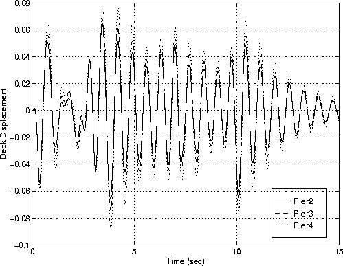
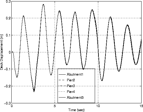
As expected, the isolated bridge undergoes larger displacements than the non-isolated bridge. For example, at Pier 4 the maximum displacement of the isolated bridge is about 3.2 times larger than the maximum displacement of the non-isolated bridge (see Figures 8 and 9). Also notice that because the isolators undergo nonlinear deformations, the isolated bridge has a 0.02 m residual displacement after the earthquake response has ceased.
Capacity design principles for base isolated bridges dictate that hysteretic energy dissipation should be confined to the isolation system. Only under extreme circumstances should the piers deform into the inelastic range.
Figure 10 shows the force-displacement response of a typical isolator, in this case, the isolator at Pier 4.
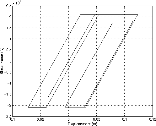
The isolator ductility "mu_d" may be defined as:
            delta_p
    mu_d = -------- + 1
           delta_de
Here "delta_de" and "delta_p" are the elastic and plastic deformation components of the isolator, respectively (hence, the total isolator displacement is "delta_de + delta_p").
The effective ductility for the combined pier-isolator system is:
                 delta_p
    mu_g = ------------------ + 1
           delta_s + delta_de
where "delta_de" and "delta_p" are as previously defined, and "delta_s" is the elastic deformation of the pier.
With this notion in place, Table 2 summarizes the isolator and pier-isolator ductility demands occurring at the bridge abutments and pier supports.
| Ductility | Abutments 1, 5 | Pier 2 | Pier 3 | Pier 4 |
| mu_d | 1.41 | 1.64 | 1.45 | 2.78 |
| mu_g | 1.41 | 1.42 | 1.41 | 1.40 |
The important point to note is that by designing the individual isolators for different ductility demands, the overall bridge system can be designed so that the ductilty demand on the pier-isolator system is about the same. This design strategy helps to regularize the structural response.
Figure 11 shows components of strain energy (Joules) versus time (sec) for the isolated bridge. The dashed line shows the time-variation in plastic strain-energy (or hysteretic energy) dissipated by the isolators. The solid line shows the time-variation in total strain energy for the isolated bridge.
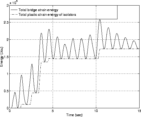
The difference between the solid and dashed lines corresponds to the strain energy stored in the bridge piers and deck.
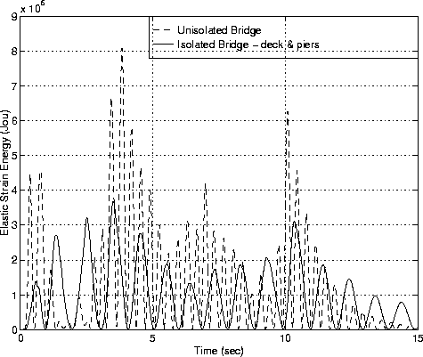
Figure 12 compares the strain energy in the deck and piers for the isolated and non-isolated structures. Because the strain energy components are roughly proportional to the square of the bridge displacements, higher strain levels of energy in the bridge components means higher possibility of damage. Figure 12 clearly shows that the peak values of strain energy in the isolated bridge deck are lower than those in the conventionally supported bridge deck. Hence, we conclude that the isolation system protects the bridge superstructure, as required.
References